


本文记录的diffusers的用法为版本0.17.0的,不同版本可能会有所不同.
VAE
VAE编码器输入
VAE的载入方式为:
from diffusers import AutoencoderKL
pretrained_model_path = 'XXX/runwayml/stable-diffusion-v1-5'   # 你下载的模型路径
vae = AutoencoderKL.from_pretrained(pretrained_model_path, subfolder = 'vae', revision = None).cuda()
上面的代码就可以载入VAE模型,VAE模型可以将图像从pixel space压缩到latent space。但是VAE接受的图像输入格式也是有一定限制的。
对于一张PIL格式的图像,可以使用diffusers自带的库将其进行处理:
from diffusers.image_processor import VaeImageProcessor
vae_scale_factor = 2 ** (len(vae.config.block_out_channels) - 1)
vae_image_processor = VaeImageProcessor(vae_scale_factor=vae_scale_factor, do_convert_rgb=True, do_normalize=True)

# image: PIL type
image0 = vae_image_processor.preprocess(image, height=512, width=512).to(device=vae.device)
image1 = vae_image_processor.preprocess(image).to(device=vae.device)
vae_image_processor可以将PIL图像和VAE的输入格式进行相互转化,接下来我们来说一下各个参数的详细情况。
- vae_scale_factor: 保证输入的图像必须为该变量的整数倍尺寸,如果不足整数倍,则需要将图像resize到整数倍的尺寸。这是因为VAE是encoder-decoder格式的,会对图像进行二倍下采样和上采样操作,因此需要是2的整数倍。默认为8
- do_normalize:决定图像是否会经过正则化操作。正则化操作为将图像经过2x-1变换由[0,1]变换为[-1,1]之间。如果输入的图像最小值小于0,那就不经过该变换。默认为True
- height & width:如果这两项未定义,那么就会按照原图像的尺寸进行保留,如果尺寸被定义,那么就会resize到定义的尺寸。
随后resize后的图像被转化为torch.tensor的格式。
了解了以上的操作之后,我们可以按一下上面两个变换的输出尺寸,类型等情况:
print(image.size)
print(image0.shape,image0.dtype,image0.max(),image0.min())
print(image1.shape, image1.dtype, image1.max(), image1.min())

# output
(1032, 1611)
torch.Size([1, 3, 512, 512]) torch.float32 tensor(1., device='cuda:1') tensor(-1., device='cuda:1')
torch.Size([1, 3, 1608, 1032]) torch.float32 tensor(1., device='cuda:1') tensor(-1., device='cuda:1')
可以看到指定尺寸的被resize到了512*512,而未规定尺寸的还是原图的尺寸,但是被调整到了8的整数倍,因此稍有些不一样。
由此就得到了VAE编码器的输入形式,如果不想使用vae_image_processor来进行预处理的话,那么也可以自己根据以上格式自行编写。
VAE编码器
接下来就可以将载入的vae模型来编码处理好的图像格式了,处理好的格式如下所示:
latent0 = vae.encode(image0).latent_dist.sample()
latent1 = vae.encode(image1).latent_dist.sample()
print(latent0.shape, latent0.dtype, latent0.max(), latent0.min())
print(latent1.shape, latent1.dtype, latent1.max(), latent1.min())


# output
torch.Size([1, 4, 64, 64]) torch.float32 tensor(27.4057, device='cuda:1') tensor(-31.7274, device='cuda:1')
torch.Size([1, 4, 201, 129]) torch.float32 tensor(45.3792, device='cuda:1') tensor(-55.3543, device='cuda:1')
由此可见,图像通道变成了4通道,图像的宽高变为了原来的八分之一,由pixel space变为了latent space。
那么encode的具体操作是怎么样的呢?代码如下:
path : src/diffusers/models/autoencoder_kl.py   160行
h = self.encoder(x)
moments = self.quant_conv(h)
posterior = DiagonalGaussianDistribution(moments)
首先将输入图像经过encoder网络结构,这个时候latent的维度为[1,8,h,w],随后的quant-conv层是一个单层卷积,不改变图像维度和尺寸,得到moments的维度也是[1,8,h,w]。posterior是一个类,会先使用torch.chunk将moments按照维度拆分为mean和logvar,维度都是[1,4,h,w],分别代表均值和log的方差,标准差为std = torch.exp(0.5 * logvar)。因此加噪过程为mean+N(0,1)*std,这个时候latent变成了一个分布,均值为mean,标准差为std的高斯分布。
如果不想得到一个分布,那么只需要一行代码即可得到隐向量,这个隐向量就是均值。
latent = torch.chunk(vae.quant_conv(vae.encoder(image)),2,dim=1)[0]VAE解码
对VAE解码则正好相反的过程。
对上述的latent进行解码的代码为:
pred0 = vae.decode(latent0, return_dict=False)[0]
pred1 = vae.decode(latent1, return_dict=False)[0]

# output
torch.Size([1, 3, 512, 512]) torch.float32 tensor(1.0408, device='cuda:1') tensor(-1.1240, device='cuda:1')
torch.Size([1, 3, 1608, 1032]) torch.float32 tensor(1.2434, device='cuda:1') tensor(-1.2150, device='cuda:1')
解码之后按理应该在[-1,1]之间,VAE并不是无损的编解码,因此可能会超出范围。
得到tensor之后就可以自行恢复为PIL图像啦!
Scheduler
在训练过程中,一般要给latent加噪,加噪过程diffusers也已经实现了。
假设已经得到了均值为mean,标准差为std的高斯分布latent,对latent加噪过程为:
from diffusers import PNDMScheduler
noise_scheduler = PNDMScheduler.from_pretrained(pretrained_model_path, subfolder="scheduler")
timesteps = torch.randint(0, noise_scheduler.config.num_train_timesteps, (bsz,), device=latents.device)
timesteps = timesteps.long()
latents = latents * vae.config.scaling_factor
noise = torch.randn_like(latents)
noisy_latents = noise_scheduler.add_noise(latents, noise, timesteps)
首先要载入scheduler,随后随机选择一个时间t来对latents进行加噪,这里有一些超参数需要特别说明一下:
- num_train_timesteps:1000,也就是加噪的最大步数。t的范围为[0,1000)
- scaling_factor: 0.18215.进行一个尺度的缩放。因为pixel space变成latent space之后的值都特别大,因此需要一个缩放因子来让范围变小。
缩放后的范围如下:
latent0 = latent0 * vae.config.scaling_factor
print(latent0.max(), latent0.min())

# output
tensor(4.9919, device='cuda:1') tensor(-5.7792, device='cuda:1')
至于为什么没有缩放到[-1,1]之间呢?我也不知道。欢迎大佬解答。
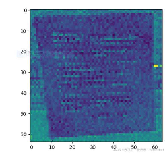
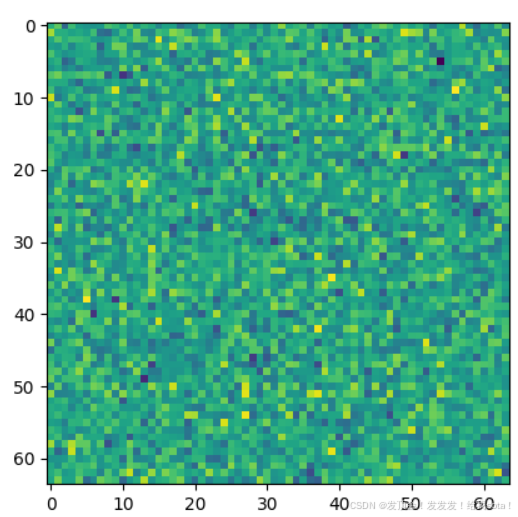
上面两个图就是未加噪的latent和加噪1000步之后的latent。肉眼来看确实是看不出原来的信息了。
UNet
Unet会对上述加噪后的latent进行去噪,代码为:
noise_scheduler.set_timesteps(args.num_inference_steps, device=vae.device)
timesteps = noise_scheduler.timesteps
timesteps = timesteps.long()
for i, t in enumerate(timesteps):
    noise_pred = unet(latents,
                      t,
                      encoder_hidden_states=prompt_embeds,
                      down_block_additional_residuals= down_block_res_samples,
                      ).sample

    latents = noise_scheduler.step(noise_pred, t, latents, return_dict=False)[0]
我一般常用的命令如上所示。
虽然加噪是1000步,但是实际上可以跳步去噪,只需要设置好相应的时间步即可。
latents为加噪t步的隐变量,t则是代表当前时间步。
因为我用的是condition的扩散模型,那么给的prompt经过编码之后为A,传给encoder_hidden_states,作为控制diffusion生成的条件,整合的方式为cross attention。prompt编码之后的维度应该为[b, seq_length, 768].
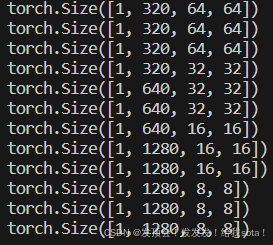
而down_block_additional_residuals则作为额外的unet decoder信息。在传统的unet中,使用skip connection连接,decoder每一层的输入为上一层的输出与encoder对应层的输出的concatenate,而有了down_block_additional_residuals之后,decoder每一层的输入为上一层的输出与encoder对应层的输出+down_block_additional_residuals的和的串联。相当于提供了额外的生成信息,从而对扩散模型有了更多的控制条件。为了匹配每一层encoder的输出,我也打印了出来,后续如果微调需要将这些维度变成一样的。
由此模型会预测每一步的噪声,然后使用step步骤根据x_t,epsilon_t转换得到x_{t-1}.
最终解码得到的隐向量示意图为:
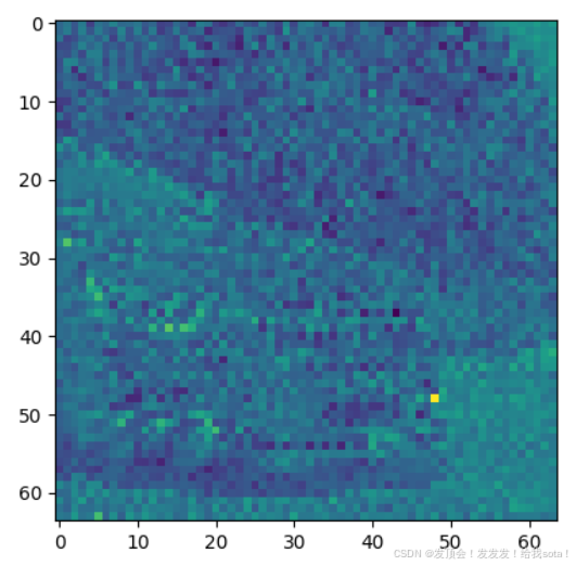
这里我用的prompt embed为全0的矩阵,尺度为[1,100,768],因为没有提供任何引导信息,因此解码出来的东西肯定和原来不一样,但是i实际上已经有了语义信息,和上面的噪声图明显不一样。


 899
899

 被折叠的 条评论
为什么被折叠?
被折叠的 条评论
为什么被折叠?
 到【灌水乐园】发言


