学会这个短线分析小技巧，轻松提升你的投资组合收益！（附源码）

作者：老余捞鱼

原创不易，转载请标明出处及原作者。

写在前面的话：本文将带您探索如何通过短线分析优化投资策略，利用支撑位和阻力位分析提升股票组合表现。通过Python代码示例，将为您展示具体操作方法，并阐述如何计算交易净收益。这些技巧能帮助投资者在管理投资组合时更加高效和精准。

概述

假设您已经有了一个长期的股票投资组合——可能是听了某个厉害的分析师的建议，或者你自己研究了一番后选的。你还打算未来很长一段时间都拿着这个股票组合不动。不过，就像所有聪明的投资者一样，你也许会时不时地调整一下，让投资组合的风险和收益保持在一个你觉得最舒服的状态。

一般来说，你可能会用到一些工具，比如公允价值估算、目标价格或者蒙特卡罗模拟来帮你决定每只股票该买多少。这些方法确实能帮你判断哪些股票值得留着，以及每只股票该占多少比例。不过，当你打算加仓或者减仓的时候（比如往投资组合里加钱，或者在调整时卖掉一部分），短期的技术分析也能给你一些额外的参考。特别是看看股票的支撑位和阻力位，能让你知道它现在的位置离最近的高点或低点有多远——这些信息对你调整买卖点很有帮助，而且不会影响你长期的持股计划。

接下来，我会一步步教你如何系统地找出支撑位和阻力位，模拟一些假设的交易，最后生成一个清晰易懂的数据表格。这个表格不仅会列出交易细节，还会包含一个“最新检测”的快照。这个快照能告诉你哪些股票现在可能接近支撑位或阻力位——这些信息可能会影响你下次调整投资组合时的资金分配。

步骤 1：设置和数据下载

下面是一个简单的设置脚本，用来定义一些核心参数，并从雅虎财经获取数据。这些参数包括：

• STOP_LOSS：10% 的名义阈值，在我们的示例情景中，如果市场走势对假设头寸不利，则强制退出。
• 税率：对盈利交易扣税 15%，以模拟现实世界中净收益的税收影响。

import pandas as pd
import numpy as np
import yfinance as yf
from datetime import datetime
import matplotlib.pyplot as plt
import seaborn as sns

START_DATE = "2020-09-01"
END_DATE = "2025-01-01"
INTERVAL = "1d"

STOP_LOSS = 0.10  # 10% hypothetical stop loss
TAX_RATE = 0.15   # 15% tax rate on gains

# Example: a portfolio of 10 stocks already held for the long term
symbols = [
    "PRIO3.SA", "ITUB4.SA", "VALE3.SA", "ABEV3.SA",
    "RENT3.SA", "WEGE3.SA", "B3SA3.SA", "JBSS3.SA",
    "VIVT3.SA", "EGIE3.SA"
]

为便于演示，我们挑选了十只股票（以 .SA 结尾）。实际上，您可以将同样的逻辑应用于您拥有的任何一组股票或 ETF。

步骤 2：检测局部最小值和最大值

下面是将贯穿我们整个代码的三个辅助函数：

def is_local_min(df, idx):
    window_lows = df['Low'].iloc[idx-2 : idx+3]
    return df['Low'].iloc[idx] == window_lows.min()

def is_local_max(df, idx):
    window_highs = df['High'].iloc[idx-2 : idx+3]
    return df['High'].iloc[idx] == window_highs.max()

def sufficiently_far(new_price, accepted_prices, threshold):
    return all(abs(new_price - ap) > threshold for ap in accepted_prices)

• is_local_max：对 "High"值进行反向操作，将其标记为阻力。
• sufficiently_far：为了避免记录过于接近的多个水平，我们会用最近的平均K线高度作为“阈值”（threshold）。这样可以确保大家只关注那些有意义的支撑位和阻力位，而不是那些过于接近、可能没什么参考价值的水平。

本地最小值/最大值示例

• 如果您有 [D-2、D-1、D、D+1、D+2] 天的价格 [10.00、9.80、9.75、9.84、9.90]，那么 D 天的低点 9.75 可能符合本地支撑条件--因为它是该 5 天窗口中的最低点。
• 相反，如果 D 日是这 5 天内的最高点，则会被标记为阻力位。

步骤 3：构建数据框并筛选支撑位/阻力位

建立一个结构来存储分析结果——既包括假设的交易方案，也有“最后检测”（last detection）的概览。接着为每只股票下载历史数据，标记出局部的最低点和最高点，然后过滤掉不重要的部分，只保留那些真正有参考价值的支撑位和阻力位。这样，我们就能更清晰地看到哪些位置可能对未来的交易决策有帮助。

all_trades_long = []
all_trades_short = []
last_detection_list = []

for symbol in symbols:
    data = yf.download(symbol, start=START_DATE, end=END_DATE, interval=INTERVAL)
    if data.empty:
        continue

    # Adjust multi-index if needed
    if isinstance(data.columns, pd.MultiIndex):
        data.columns = data.columns.droplevel(0)
    data.columns = ['Adj Close', 'Close', 'High', 'Low', 'Open', 'Volume']
    data.reset_index(inplace=True)

    df = data[['Date', 'Open', 'High', 'Low', 'Close']].copy()
    df['isSupport'] = False
    df['isResistance'] = False
    df['AvgCandleHeight'] = np.nan

    # Mark local minima/maxima
    for t in range(len(df)):
        j = t - 2
        if j - 2 >= 0 and j + 2 < len(df):
            if is_local_min(df, j):
                df.loc[j, 'isSupport'] = True
            if is_local_max(df, j):
                df.loc[j, 'isResistance'] = True

        # Rolling ~32-day average candle height
        window_start = max(0, t - 32 + 1)
        sub_df = df.iloc[window_start : t+1]
        if len(sub_df) > 0:
            df.loc[t, 'AvgCandleHeight'] = np.mean(sub_df['High'] - sub_df['Low'])

    # Gather raw levels
    raw_levels = []
    for i in range(len(df)):
        if df['isSupport'].iloc[i]:
            raw_levels.append({'index': i, 'price': df['Low'].iloc[i], 'type': 'support'})
        elif df['isResistance'].iloc[i]:
            raw_levels.append({'index': i, 'price': df['High'].iloc[i], 'type': 'resistance'})

    # Filter out levels that are too close
    final_levels = []
    unique_prices = []
    for lvl in raw_levels:
        idx = lvl['index']
        candle_height = df['AvgCandleHeight'].iloc[idx]
        if np.isnan(candle_height):
            continue
        if sufficiently_far(lvl['price'], unique_prices, candle_height):
            final_levels.append(lvl)
            unique_prices.append(lvl['price'])

假设平均K线高度是 0.50 美元，而且我们已经确定了 20.00 美元是一个支撑位。如果接下来又出现了一个潜在的支撑位，比如 20.10 美元，我们会计算它与之前支撑位的距离。如果 abs(20.10 - 20.00) < 0.50，也就是说两者差距小于 0.50 美元，那可能会忽略这个新的支撑位。这样一来，就能避免在图表上标记出太多几乎相同的水平线，让最终的支撑位和阻力位更加清晰、更有参考价值。

步骤 4：记录 "最后检测"（Last Detection）

对于每个符号，我们都会查看最近（上次）确定的支撑位/阻力位。这在您决定当前价格是否是支撑位/阻力位时尤为重要：

• 高于近期支撑位（或许是个好兆头，或高于该支撑位 ~5%）。
• 低于近期阻力位（例如，如果阻力位下仅有-3%，可能要谨慎）。

    if len(final_levels) > 0:
        last_level = final_levels[-1]
        last_detection_idx = last_level['index']
        last_detection_date = df['Date'].iloc[last_detection_idx]
        last_detection_price = last_level['price']
        last_close_price = df['Close'].iloc[-1]

        diff_rel = (last_close_price / last_detection_price) - 1.0

        last_detection_list.append({
            'symbol': symbol,
            'last_detection_type': last_level['type'],
            'last_detection_date': last_detection_date.strftime('%Y-%m-%d'),
            'last_detection_price': round(last_detection_price, 2),
            'last_date': df['Date'].iloc[-1].strftime('%Y-%m-%d'),
            'last_close_price': round(last_close_price, 2),
            'diff_relative (%)': round(diff_rel * 100, 2)
        })

快速示例

如果上一次检测到的支撑位是 30 美元，而最终收盘价是 33 美元，那么diff_relative (%)大约为 +10%。这可能表明，该股在其最近的支撑位上方处于舒适的位置。从再平衡的角度来说，你可以把它理解为 "该股最近从支撑位反弹"，这可能是你决策过程的一部分。

步骤 5： "Long"和 "Short"方案

我们模拟了两种假设方法，以说明在投资管理中如何使用这些支撑位/阻力位：

• 在支撑位后 3 天买入（做多），在下一个阻力位后 3 天卖出。
• 在阻力位后 3 天做空（卖出），在下一个支撑位后 3 天买回来。

3 天的延迟并不是随便定的——这是因为我们需要多观察 2 天，才能确认某一天的价格是不是局部的最低点或最高点。换句话说，只有等到第 3 天，我们才能有足够的依据来判断是否真的出现了支撑位或阻力位，然后才能决定是否采取行动。这样做的目的是为了避免误判，确保我们的分析更准确。

长期（Long）战略示例

    trades_long = []
    for i in range(len(final_levels) - 1):
        if final_levels[i]['type'] == 'support' and final_levels[i+1]['type'] == 'resistance':
            support_idx = final_levels[i]['index']
            resistance_idx = final_levels[i+1]['index']
            if resistance_idx <= support_idx:
                continue

            real_entry_idx = support_idx + 3
            real_exit_idx = resistance_idx + 3
            if real_entry_idx >= len(df) or real_exit_idx >= len(df):
                continue

            real_entry_price = df['Close'].iloc[real_entry_idx]
            real_exit_price = df['Close'].iloc[real_exit_idx]

            # Hypothetical 10% stop-loss
            max_loss_price = real_entry_price * (1 - STOP_LOSS)
            slice_min = df['Low'].iloc[real_entry_idx : real_exit_idx+1].min()
            if slice_min < max_loss_price:
                stop_day = df['Low'].iloc[real_entry_idx : real_exit_idx+1].idxmin()
                real_exit_idx = stop_day
                real_exit_price = max_loss_price

            gross_return = (real_exit_price / real_entry_price) - 1.0
            net_return = gross_return * (1 - TAX_RATE) if gross_return > 0 else gross_return

            support_price = final_levels[i]['price']
            resistance_price = final_levels[i+1]['price']
            entry_vs_support_pct_diff = (real_entry_price / support_price) - 1.0
            exit_vs_resistance_pct_diff = (real_exit_price / resistance_price) - 1.0
            trade_days = (df['Date'].iloc[real_exit_idx] - df['Date'].iloc[real_entry_idx]).days
            daily_net_return = (1 + net_return)**(1 / trade_days) - 1 if trade_days > 0 else 0.0

            trades_long.append({
                'support_date': df['Date'].iloc[support_idx].strftime('%Y-%m-%d'),
                'resistance_date': df['Date'].iloc[resistance_idx].strftime('%Y-%m-%d'),
                'support_price': round(support_price, 2),
                'resistance_price': round(resistance_price, 2),
                'real_entry_date': df['Date'].iloc[real_entry_idx].strftime('%Y-%m-%d'),
                'real_exit_date': df['Date'].iloc[real_exit_idx].strftime('%Y-%m-%d'),
                'real_entry_price': round(real_entry_price, 2),
                'real_exit_price': round(real_exit_price, 2),
                'entry_vs_support_pct_diff': round(entry_vs_support_pct_diff * 100, 2),
                'exit_vs_resistance_pct_diff': round(exit_vs_resistance_pct_diff * 100, 2),
                'gross_return (%)': round(gross_return * 100, 2),
                'net_return (%)': round(net_return * 100, 2),
                'daily_net_return (%)': round(daily_net_return * 100, 2),
                'symbol': symbol
            })

    all_trades_long.extend(trades_long)

在实际的投资管理中，这种做法可能相当于：当你发现某只股票的价格明显触底（支撑位）时，考虑是否要加仓；而当价格接近顶部（阻力位）时，考虑是否要减仓，降低风险。

不过，这些操作只是作为长期投资策略的补充，目的是在保持长期持仓的同时，利用短期的市场波动来优化收益和风险。

短期（Short）策略示例

    trades_short = []
    for i in range(len(final_levels) - 1):
        if final_levels[i]['type'] == 'resistance' and final_levels[i+1]['type'] == 'support':
            resistance_idx = final_levels[i]['index']
            support_idx = final_levels[i+1]['index']
            if support_idx <= resistance_idx:
                continue

            real_entry_idx = resistance_idx + 3
            real_exit_idx = support_idx + 3
            if real_entry_idx >= len(df) or real_exit_idx >= len(df):
                continue

            real_entry_price = df['Close'].iloc[real_entry_idx]
            real_exit_price = df['Close'].iloc[real_exit_idx]

            # 10% stop-loss if price rises
            max_loss_price = real_entry_price * (1 + STOP_LOSS)
            slice_max = df['High'].iloc[real_entry_idx : real_exit_idx+1].max()
            if slice_max > max_loss_price:
                stop_day = df['High'].iloc[real_entry_idx : real_exit_idx+1].idxmax()
                real_exit_idx = stop_day
                real_exit_price = max_loss_price

            gross_return = (real_entry_price - real_exit_price) / real_entry_price
            net_return = gross_return * (1 - TAX_RATE) if gross_return > 0 else gross_return

            resistance_price = final_levels[i]['price']
            support_price = final_levels[i+1]['price']
            entry_vs_resistance_pct_diff = (real_entry_price / resistance_price) - 1.0
            exit_vs_support_pct_diff = (real_exit_price / support_price) - 1.0
            trade_days = (df['Date'].iloc[real_exit_idx] - df['Date'].iloc[real_entry_idx]).days
            daily_net_return = (1 + net_return)**(1 / trade_days) - 1 if trade_days > 0 else 0.0

            trades_short.append({
                'resistance_date': df['Date'].iloc[resistance_idx].strftime('%Y-%m-%d'),
                'support_date': df['Date'].iloc[support_idx].strftime('%Y-%m-%d'),
                'resistance_price': round(resistance_price, 2),
                'support_price': round(support_price, 2),
                'real_entry_date': df['Date'].iloc[real_entry_idx].strftime('%Y-%m-%d'),
                'real_exit_date': df['Date'].iloc[real_exit_idx].strftime('%Y-%m-%d'),
                'real_entry_price': round(real_entry_price, 2),
                'real_exit_price': round(real_exit_price, 2),
                'entry_vs_resistance_pct_diff': round(entry_vs_resistance_pct_diff * 100, 2),
                'exit_vs_support_pct_diff': round(exit_vs_support_pct_diff * 100, 2),
                'gross_return (%)': round(gross_return * 100, 2),
                'net_return (%)': round(net_return * 100, 2),
                'daily_net_return (%)': round(daily_net_return * 100, 2),
                'symbol': symbol
            })

    all_trades_short.extend(trades_short)

虽然做空（空头头寸）通常不是长期、基本面驱动的投资组合的常见操作，但了解这些信号仍然很有用。比如，如果一只股票多次在某个阻力位附近掉头下跌，你可能会更愿意等待一个更好的买入机会，而不是在接近阻力位的时候加仓。这样一来，你就能避免在高点附近买入，降低短期风险，同时依然保持对长期投资的信心。

步骤 6：合并和解释结果

当我们处理完所有股票后，会分别创建“多头”和“空头”交易的 DataFrames，然后计算每只股票的相关统计数据，比如正净收益的概率、价格与支撑位/阻力位的平均差距等。接着，把这些统计数据整合到最后检测数据集（last_detection_df）中，这样每只股票都会有一个清晰的快照，方便你快速了解它的当前状态和潜在交易机会。

trade_results_long = pd.DataFrame(all_trades_long)
trade_results_short = pd.DataFrame(all_trades_short)

# Probability of net return > 0, etc.
if not trade_results_long.empty:
    group_long = trade_results_long.groupby('symbol')
    df_long_metrics = group_long.agg({
        'net_return (%)': lambda x: np.mean(x > 0) * 100,
        'entry_vs_support_pct_diff': 'mean'
    }).reset_index()
    df_long_metrics.rename(columns={
        'net_return (%)': 'prob_win_long (%)',
        'entry_vs_support_pct_diff': 'avg_entry_vs_support_pct_diff'
    }, inplace=True)
else:
    df_long_metrics = pd.DataFrame(columns=['symbol','prob_win_long (%)','avg_entry_vs_support_pct_diff'])

if not trade_results_short.empty:
    group_short = trade_results_short.groupby('symbol')
    df_short_metrics = group_short.agg({
        'net_return (%)': lambda x: np.mean(x > 0) * 100,
        'entry_vs_resistance_pct_diff': 'mean'
    }).reset_index()
    df_short_metrics.rename(columns={
        'net_return (%)': 'prob_win_short (%)',
        'entry_vs_resistance_pct_diff': 'avg_entry_vs_resistance_pct_diff'
    }, inplace=True)
else:
    df_short_metrics = pd.DataFrame(columns=['symbol','prob_win_short (%)','avg_entry_vs_resistance_pct_diff'])

df_merged_metrics = pd.merge(df_long_metrics, df_short_metrics, on='symbol', how='outer')

last_detection_df = pd.DataFrame(last_detection_list)
last_detection_df = pd.merge(last_detection_df, df_merged_metrics, on='symbol', how='left')

last_detection_df.rename(columns={
    'prob_win_long (%)': 'prob_win_long',
    'avg_entry_vs_support_pct_diff': 'avg_entry_vs_support_pct_diff',
    'prob_win_short (%)': 'prob_win_short',
    'avg_entry_vs_resistance_pct_diff': 'avg_entry_vs_resistance_pct_diff'
}, inplace=True)

last_detection_df[['prob_win_long','avg_entry_vs_support_pct_diff',
                   'prob_win_short','avg_entry_vs_resistance_pct_diff']] = \
    round(last_detection_df[['prob_win_long','avg_entry_vs_support_pct_diff',
                       'prob_win_short','avg_entry_vs_resistance_pct_diff']].fillna(0), 2)

最后，我们可以对表格进行检查：

print("=== TRADE RESULTS (LONG) ===\n")
print(trade_results_long)

print("\n=== TRADE RESULTS (SHORT) ===\n")
print(trade_results_short)

print("\n=== LAST DETECTION DF ===\n")
print(last_detection_df)

步骤 7：输出结果

从样本数据来看，我们可能会发现有 63 笔“多头”交易和 62 笔“空头”交易。更重要的是，last_detection_df 会显示每只股票最近的支撑位或阻力位事件，以及当前收盘价与这些关键水平的关系。举个例子，如果某只股票的收盘价接近支撑位，这可能是一个潜在的买入机会；而如果它接近阻力位，则可能意味着需要谨慎，甚至考虑减仓。这个数据集能帮你快速判断每只股票的当前状态，为下一步操作提供参考。

• last_detection_type 的支撑价为 29.72 美元（2024-12-18）；
• last_close_price（最后收盘价）为 32.20 美元；
• diff_relative (%) 为 +8.34。

这表明股价比最近的支撑位高出约 8.34%--可能是短期势头稳定的迹象。另一个符号可能会出现阻力检测，价格在该阻力位下-16.15%，表明股价可能从高位区域回落。

还请注意 prob_win_long 和 prob_win_short两栏，它们反映了在 "做多 "或 "做空 "模拟中，每个符号的假设净收益以正数结束的频率（以百分比表示）。如果某个股票的多头概率较高（例如 66.7%），则表示我们模拟的该股票多头交易在扣除税款和止损检查后通常都能获得收益。与此同时，如果某个股票的赢利概率（prob_win_short）较高，则表明该股票经常从局部最大值回撤，因为这些假定的 "空头 "交易在一半以上的时间里都能获得正收益。

下面是最终输出结果的示例片段：

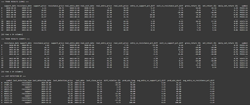
请注意，不同符号的 prob_win_long 和 prob_win_short 差异很大。您可能会发现，像 ABEV3.SA 这样的股票，其概率_win_short 为 80%，这表明在我们的模拟中，它经常会从局部峰值回调；而像 RENT3.SA 这样的股票，其概率_win_long 为 80%，这表明它往往会从支撑位反弹。

步骤 8：添加视觉元素（概率与分布）

为了快速了解这些概率，我们可以绘制简单的计量图，比较正净收益的比例（所有多头交易与所有空头交易的比例）。要想获得更精细的视图，还可以按符号绘制每日净回报的“小提琴图”。下面是一个示例，说明如何创建两个并排的计量图，一个是多头概率汇总图，另一个是空头概率汇总图：

import numpy as np
import matplotlib.pyplot as plt
import seaborn as sns

positive_returns_long = trade_results_long['daily_net_return (%)'] > 0
probability_positive_long = positive_returns_long.mean()

positive_returns_short = trade_results_short['daily_net_return (%)'] > 0
probability_positive_short = positive_returns_short.mean()

# --- 1) Gauge Charts Side by Side ---
fig, (ax1, ax2) = plt.subplots(1, 2, figsize=(20, 1.5))

# Left: LONG
color_long = 'green' if probability_positive_long > 0.5 else 'red'
ax1.barh([0], [probability_positive_long], color=color_long, height=0.4, alpha=0.8)
ax1.barh([0], [0.5], color='gray', height=0.4, alpha=0.3)
ax1.set_xlim(0, 1)
ax1.set_yticks([])
ax1.set_xticks(np.linspace(0, 1, 11))
ax1.set_xticklabels([f"{int(x*100)}%" for x in np.linspace(0, 1, 11)], fontsize=9)
ax1.set_title('Prob. Daily Return > 0 (LONG)', fontsize=10, fontweight='bold')
ax1.axvline(0.5, color='black', linestyle='--', alpha=0.7)
ax1.text(probability_positive_long, 0.05, f"{probability_positive_long:.1%}",
         ha='center', fontsize=10, fontweight='bold', color='black')

# Right: SHORT
color_short = 'green' if probability_positive_short > 0.5 else 'red'
ax2.barh([0], [probability_positive_short], color=color_short, height=0.4, alpha=0.8)
ax2.barh([0], [0.5], color='gray', height=0.4, alpha=0.3)
ax2.set_xlim(0, 1)
ax2.set_yticks([])
ax2.set_xticks(np.linspace(0, 1, 11))
ax2.set_xticklabels([f"{int(x*100)}%" for x in np.linspace(0, 1, 11)], fontsize=9)
ax2.set_title('Prob. Daily Return > 0 (SHORT)', fontsize=10, fontweight='bold')
ax2.axvline(0.5, color='black', linestyle='--', alpha=0.7)
ax2.text(probability_positive_short, 0.05, f"{probability_positive_short:.1%}",
         ha='center', fontsize=10, fontweight='bold', color='black')

plt.tight_layout()
plt.show()

还能直观显示按符号划分的每日净收益分布：

# --- 2) Violin Plots Side by Side ---
fig, (ax1, ax2) = plt.subplots(1, 2, figsize=(20, 6))

# Left: LONG Distribution
sns.violinplot(
    data=trade_results_long,
    x='symbol',
    y='daily_net_return (%)',
    hue='symbol',
    palette='muted',
    inner='box',
    ax=ax1
)
ax1.set_title('Distribution of Daily Returns (LONG)', fontsize=14, fontweight='bold')
ax1.set_xlabel('Asset', fontsize=12)
ax1.set_ylabel('Net Daily Return (%)', fontsize=12)
ax1.tick_params(axis='x', rotation=45, labelsize=10)
ax1.tick_params(axis='y', labelsize=10)
ax1.grid(axis='y', linestyle='--', alpha=0.7)

# Right: SHORT Distribution
sns.violinplot(
    data=trade_results_short,
    x='symbol',
    y='daily_net_return (%)',
    hue='symbol',
    palette='muted',
    inner='box',
    ax=ax2
)
ax2.set_title('Distribution of Daily Returns (SHORT)', fontsize=14, fontweight='bold')
ax2.set_xlabel('Asset', fontsize=12)
ax2.set_ylabel('Net Daily Return (%)', fontsize=12)
ax2.tick_params(axis='x', rotation=45, labelsize=10)
ax2.tick_params(axis='y', labelsize=10)
ax2.grid(axis='y', linestyle='--', alpha=0.7)

plt.tight_layout()
plt.show()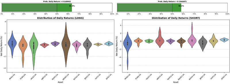

这些图揭示了哪些股票的日收益率范围更窄、更一致（短期内可能更稳定），哪些股票的波动更大或尾部更长。如果一个符号的长线小提琴图具有明显的正偏斜，这可能与较高的长线赢利概率（prob_win_long）相一致，从而强化了 "在支撑位附近买入 "的短期方案一般都能奏效的观点--这在决定投资组合配置时是很有价值的。

观点总结

• 通过系统地分析支撑位和阻力位，并模拟假设的交易结果（包括税后净收益和止损点），你可以为长期投资组合的调整和资金分配提供额外的参考。
• 这种方法并不会取代你的基本面分析或蒙特卡洛模拟策略，而是为你提供了一种新的视角，帮助你更好地了解每只股票当前的价格相对于近期关键转折点的位置。
• 在实际操作中，这些信息可能会影响你如何分配新资金或调整现有仓位，比如在接近支撑位时加仓，或者在接近阻力位时减仓，从而优化你的投资组合表现。

如需获取完整代码及更多详细资料，欢迎访问我的GitHub仓库。您可以根据自身投资策略的需求，自由调整、测试并整合这些短期交易信号，以优化您的投资决策流程。

地址：Stocks2025/evalPortfolio/Supercharge_AssetRebalancing.ipynb at master · alexyu2013/Stocks2025 · GitHub

感谢您阅读到最后，希望这篇文章为您带来了新的启发和实用的知识！如果觉得有帮助，请不吝点赞和分享，您的支持是我持续创作的动力。祝您投资顺利，收益长虹！如果对文中内容有任何疑问，欢迎留言，我会尽快回复！

---

本文内容仅限技术探讨和学习，不构成任何投资建议。