基于TensorFlow的机器学习(2) -- 回归模型

两种典型的回归模型是linear regression 和 logistic regression。 以下将分别对两种回归模型进行分析以及基于tensorflow的实现。

Linear Regression(线性回归)

线性回归基本概念

之前基于吴恩达的《机器学习》课程写过相关的线性回归笔记，详情可以看这里。

接下来将简单地对线性回归模型进行分析：

线性回归就是采用最小二乘法对数据点进行线性拟合(Over)。

以下是线性回归的tensorflow实现：

导入必要内容

import tensorflow as tf
import numpy
import matplotlib.pyplot as plt
rng = numpy.random

设置超参数

# Parameters
learning_rate = 0.01
training_epochs = 1000
display_step = 50

其中learning_rate表示学习率, training_epochs 表示的是运算的总次数， display_step 设置的是运行了多长时间答应一次当前各参数基本情况。

提供训练数据

# Training Data
train_X = numpy.asarray([3.3,4.4,5.5,6.71,6.93,4.168,9.779,6.182,7.59,2.167,
            7.042,10.791,5.313,7.997,5.654,9.27,3.1])

train_Y = numpy.asarray([1.7,2.76,2.09,3.19,1.694,1.573,3.366,2.596,2.53,1.221,
            2.827,3.465,1.65,2.904,2.42,2.94,1.3])

n_samples = train_X.shape[0]

其中n_samples得到的是训练数据的数量，此处为17。

构建图模型

# tf Graph Input
X = tf.placeholder("float")
Y = tf.placeholder("float")

设置模型的权值

# Set model weights
W = tf.Variable(rng.randn(), name="weight")
b = tf.Variable(rng.randn(), name="bias")
print W, b

此处采取的是随机初始化的方式，并设置初始化的类型为浮点型。

线性回归算法实现

# Construct a linear model
pred = tf.add(tf.multiply(X, W), b)

# Mean squared error
cost = tf.reduce_sum(tf.pow(pred-Y, 2))/(2*n_samples)

# Gradient descent
optimizer = tf.train.GradientDescentOptimizer(learning_rate).minimize(cost)

# Initialize the variables
init = tf.global_variables_initializer()

唯一此处有一点疑问是： 我们之前不是已经创建了初始化变量的w和b了吗，为何还要在此处对所有变量进行初始化？

模型训练

# Start training
with tf.Session() as sess:
    sess.run(init)

    # Fit all training data.
    for epoch in range(training_epochs):
        for (x, y) in zip(train_X, train_Y):
            sess.run(optimizer, feed_dict={X: x, Y: y})

        # Display logs per epoch step
        if (epoch+1) % display_step == 0:
            c = sess.run(cost, feed_dict={X: train_X, Y: train_Y})
            print "Epoch: ", "%04d" % (epoch+1), "cost=", "{:.9f}".format(c), \
                "W=", sess.run(W), "b=", sess.run(b)

    print "Optimization Finishd"
    training_cost = sess.run(cost, feed_dict={X: train_X, Y:train_Y})
    print "Training cost=", training_cost, "W=", sess.run(W), "b=", sess.run(b), '\n'

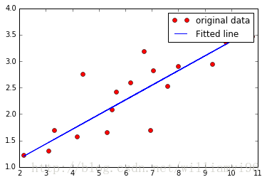
    # Graphic display
    plt.plot(train_X, train_Y, 'ro', label='original data')
    plt.plot(train_X, sess.run(W) * train_X + sess.run(b), label='Fitted line')
    plt.legend()
    plt.show()

输出结果为：

Epoch: 0050 cost= 0.102178194 W= 0.338457 b= 0.162191
Epoch: 0100 cost= 0.099263854 W= 0.333172 b= 0.200211
Epoch: 0150 cost= 0.096686281 W= 0.328201 b= 0.235971
Epoch: 0200 cost= 0.094406627 W= 0.323526 b= 0.269604
Epoch: 0250 cost= 0.092390411 W= 0.319129 b= 0.301237
Epoch: 0300 cost= 0.090607323 W= 0.314993 b= 0.330987
Epoch: 0350 cost= 0.089030363 W= 0.311103 b= 0.358969
Epoch: 0400 cost= 0.087635688 W= 0.307445 b= 0.385286
Epoch: 0450 cost= 0.086402342 W= 0.304004 b= 0.410038
Epoch: 0500 cost= 0.085311584 W= 0.300768 b= 0.433318
Epoch: 0550 cost= 0.084346980 W= 0.297725 b= 0.455214
Epoch: 0600 cost= 0.083493948 W= 0.294862 b= 0.475807
Epoch: 0650 cost= 0.082739606 W= 0.29217 b= 0.495176
Epoch: 0700 cost= 0.082072593 W= 0.289638 b= 0.513392
Epoch: 0750 cost= 0.081482716 W= 0.287256 b= 0.530526
Epoch: 0800 cost= 0.080961145 W= 0.285016 b= 0.54664
Epoch: 0850 cost= 0.080499947 W= 0.282909 b= 0.561796
Epoch: 0900 cost= 0.080092147 W= 0.280928 b= 0.576051
Epoch: 0950 cost= 0.079731591 W= 0.279064 b= 0.589458
Epoch: 1000 cost= 0.079412781 W= 0.277311 b= 0.602068
Optimization Finishd
Training cost= 0.0794128 W= 0.277311 b= 0.602068

Logistic Regression(逻辑回归)

逻辑回归基本概念

逻辑回归基本概念可以参考之前学习吴恩达《机器学习》课程的笔记。

以下是逻辑回归的tensorflow代码实现：

导入必要内容

import tensorflow as tf

# Import MNIST data
from tensorflow.examples.tutorials.mnist import input_data
mnist = input_data.read_data_sets("/tmp/data/", one_hot=True)

此处使用到了MNIST数据集, one_hot设置为True是个神马意思？？

设置超参数

# Parameters
learning_rate = 0.01
training_epochs = 25
batch_size = 100
display_step = 1

此处引入到了批处理的概念，每次迭代处理的输入图片数量为batch_size, 一共进行25次迭代，同时每次迭代都显示当前各参数的状态。

图模型输入

# tf Graph Input
x = tf.placeholder(tf.float32, [None, 784]) # mnist data image of shape 28*28=784
y = tf.placeholder(tf.float32, [None, 10]) # 0-9 digits recognition => 10 classes

# Set model weights
W = tf.Variable(tf.zeros([784, 10]))
b = tf.Variable(tf.zeros([10]))

配置逻辑回归基本数据

# Construct model
pred  = tf.nn.softmax(tf.matmul(x, W) + b) # Softmax

# Minimize error using cross entropy
cost = tf.reduce_mean(-tf.reduce_sum(y*tf.log(pred), reduction_indices=1))

# Gradient Descent
optimizer = tf.train.GradientDescentOptimizer(learning_rate).minimize(cost)

# Initialize the variables (i.e. assign their default value)
init = tf.global_variables_initializer()

此处使用到了交叉熵以及随机梯度下降两种方法，值得注意。

模型训练

# Start training
with tf.Session() as sess:
    sess.run(init)

    # Training cycle
    for epoch in range(training_epochs):
        avg_cost = 0.
        total_batch = int(mnist.train.num_examples/batch_size)
        # Loop over all batches
        for i in range(total_batch):
            batch_xs, batch_ys = mnist.train.next_batch(batch_size)
            # print mnist.train.next_batch(batch_size)

            # Fit training using batch data
            _, c = sess.run([optimizer, cost], feed_dict={x: batch_xs, y: batch_ys})

            # Compute average loss
            avg_cost += c / total_batch
        # Display logs per epoch step
        if (epoch+1) % display_step == 0:
            print "Epoch:", "%04d" % (epoch+1), "cost=", "{:.9f}".format(avg_cost)

    print "Optimization Finished"

    # Test model
    correct_prediction = tf.equal(tf.argmax(pred, 1), tf.argmax(y, 1))
    print correct_prediction
    # Calculate accuracy for 3000 examples
    accuracy = tf.reduce_mean(tf.cast(correct_prediction, tf.float32))
    print "Accuracy:" , accuracy.eval({x: mnist.test.images[:3000], y: mnist.test.labels[:3000]})

结果如下：

Epoch: 0001 cost= 1.183705997
Epoch: 0002 cost= 0.665137744
Epoch: 0003 cost= 0.553539150
Epoch: 0004 cost= 0.497606907
Epoch: 0005 cost= 0.466207787
Epoch: 0006 cost= 0.441998017
Epoch: 0007 cost= 0.425722898
Epoch: 0008 cost= 0.412529908
Epoch: 0009 cost= 0.401451499
Epoch: 0010 cost= 0.391796238
Epoch: 0011 cost= 0.385131709
Epoch: 0012 cost= 0.378347220
Epoch: 0013 cost= 0.372350214
Epoch: 0014 cost= 0.367119752
Epoch: 0015 cost= 0.362666935
Epoch: 0016 cost= 0.358102056
Epoch: 0017 cost= 0.356050571
Epoch: 0018 cost= 0.350696459
Epoch: 0019 cost= 0.348614010
Epoch: 0020 cost= 0.344936007
Epoch: 0021 cost= 0.343074091
Epoch: 0022 cost= 0.340528888
Epoch: 0023 cost= 0.337343196
Epoch: 0024 cost= 0.336431599
Epoch: 0025 cost= 0.333592685
Optimization Finished
Tensor(“Equal_2:0”, shape=(?,), dtype=bool)
Accuracy: 0.888667

以上便是关于回归模型的所有内容。