Spark 下一代机器学习教程（四）

原文：Next-Generation Machine Learning with Spark

协议：CC BY-NC-SA 4.0

六、图分析

告诉我我会死在哪里，这样我就不会去那里。

—芒格 ⁱ

图分析是一种数据分析技术，用于确定图中对象之间关系的强度和方向。图是用于建模对象之间的关系和过程的数学结构。 ⁱⁱ 它们可以用来表示数据中的复杂关系和依赖关系。图由代表系统中实体的顶点或节点组成。这些顶点由表示这些实体之间关系的边连接。 ⁱⁱⁱ

图介绍

这可能不会立即显而易见，但图无处不在。LinkedIn、脸书和 Twitter 等社交网络就是图。互联网和万维网是图。计算机网络是图。自来水管道是图。道路网络是图。GraphX 等图处理框架有专门设计的图算法和操作符来处理面向图的数据。

无向图

无向图是边没有方向的图。无向图中的边可以在两个方向上遍历，并表示一种双向关系。图 6-1 显示了一个有三个节点和三条边的无向图。iv

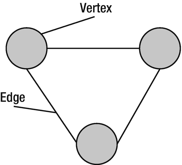
图 6-1

无向图

有向图

有向图的边的方向表示单向关系。在有向图中，每条边只能在一个方向上遍历(图 6-2 )。

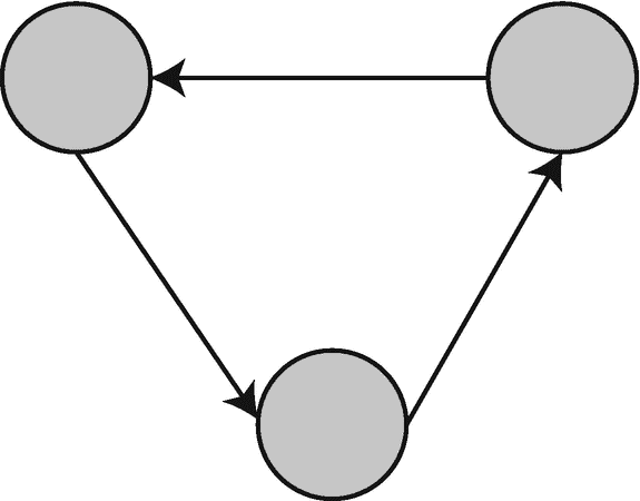
图 6-2

有向图

有向多重图

一个多重图在节点之间有多条边(图 6-3 )。

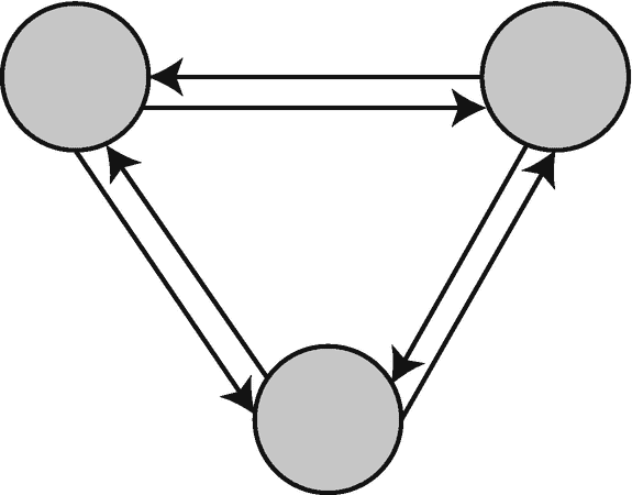
图 6-3

有向多重图

属性图

属性图是一种有向多图，其中顶点和边具有用户定义的属性 ^v (图 6-4 )。

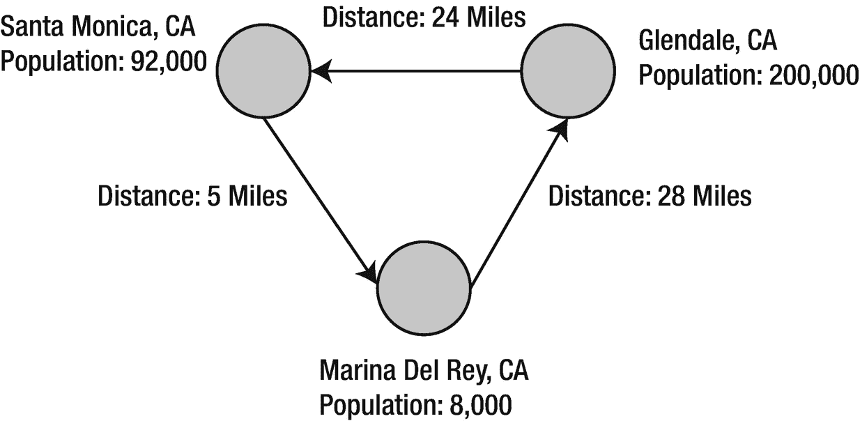
图 6-4

属性图

图分析用例

图分析已经在许多行业蓬勃发展。任何利用大量关联数据的项目都是图分析的完美用例。这并不意味着是用例的全面列表，但是它应该给你一个关于图分析的可能性的想法。

欺诈检测和反洗钱(AML)

欺诈检测和反洗钱可能是图分析最广为人知的使用案例之一。手动筛选数以百万计的银行交易来识别欺诈和洗钱活动令人望而生畏，如果不是不可能的话。通过一系列复杂的相互关联、看似无害的交易来隐藏欺诈的复杂方法加剧了这一问题。检测和防止这些类型的攻击的传统技术在今天已经变得过时了。图分析是解决这一问题的完美方法，它可以轻松地将可疑交易与其他异常行为模式联系起来。像 GraphX 这样的高性能图处理 API 允许非常快速地从一个事务到另一个事务进行复杂的遍历。这方面最著名的例子可能是巴拿马文件丑闻。通过使用图分析识别数百万份泄露文件之间的联系，分析师能够发现知名外国领导人、政治家甚至女王拥有的离岸银行账户中的隐藏资产。 ^vi

数据治理和法规遵从性

典型的大型组织将数百万个数据文件存储在中央数据存储库中，例如数据湖。这需要适当的主数据管理，这意味着每次修改文件或创建新副本时都要跟踪数据沿袭。通过跟踪数据沿袭，组织可以跟踪数据从源到目标的移动，从而了解数据从一点到另一点的所有变化方式。 ^vii 一个完善的数据沿袭策略可以增强对数据的信心，并实现准确的业务决策。数据沿袭也是维护数据相关法规遵从性的一项要求，例如通用数据保护法规(GDPR)。违反 GDPR 教被抓可能意味着巨额罚款。图分析非常适合这些用例。

风险管理

为了管理风险，对冲基金和投资银行等金融机构使用图分析来识别可能引发“黑天鹅”事件的相互关联的风险和模式。以 2008 年金融危机为例，图分析可以揭示抵押贷款支持证券(MBS)、债务抵押债券(CDO)和 CDO 部分的信用违约互换(CDs)之间错综复杂的相互依赖关系，从而让人们了解复杂的衍生品证券化过程。

运输

空中交通网络是一个图。机场代表顶点，而路线代表边。商业飞行计划是使用图分析创建的。航空公司和物流公司使用图分析进行路线优化，以确定最安全或最快的路线。这些优化确保了安全性，并且可以节省时间和金钱。

网络社交

社交网络是图分析最直观的用例。如今，几乎每个人都有一张“社交图”，它代表了一个人在社交网络中与其他人或群体的社交关系。如果你在脸书、推特、Instagram 或 LinkedIn 上，你就有了社交图谱。一个很好的例子是脸书使用 Apache Giraph，另一个开源图框架，处理和分析一万亿条边进行内容排名和推荐。 ^viii

网络基础设施管理

互联网是互联路由器、服务器、台式机、物联网和移动设备的巨大图。政府和企业网络可以被视为互联网的子图。即使是小型家庭网络也是图。设备代表顶点，网络连接代表边。图分析为网络管理员提供了可视化复杂网络拓扑的能力，这对于监控和故障排除非常有用。这对于由数千台相连设备组成的大型企业网络来说尤为重要。

GraphX 简介

GraphX 是 Spark 基于 RDD 的图处理 API。除了图操作符和算法，GraphX 还提供了存储图数据的数据类型。 ^ix

图

属性图由 graph 类的一个实例表示。就像 rdd 一样，属性图被划分并分布在执行器之间，在崩溃时可以被重新创建。属性图是不可变的，这意味着创建一个新的图对于改变图的结构或值是必要的。 ^x

VertexRDD

属性图中的顶点由 VertexRDD 表示。每个顶点只有一个条目存储在 VertexRDD 中。

边缘

edge 类包含与源和目标顶点标识符相对应的源和目标 id，以及存储 Edge 属性的属性。^Xi

边缘 d

属性图中的边由 EdgeRDD 表示。

边缘三联体

一条边和它所连接的两个顶点的组合由一个 EdgeTriplet 类的实例表示。它还包含边及其连接的顶点的属性。

边缘上下文

EdgeContext 类公开了三元组字段以及向源和目标顶点发送消息的函数。^XII

GraphX 示例

对于这个例子(清单 6-1 ，我将使用 GraphX 来分析南加州不同城市之间的距离。我们将基于表 6-1 中的数据构建一个类似图 6-5 的属性图。

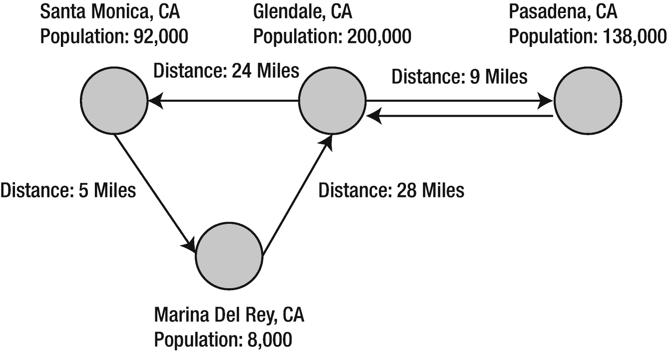
图 6-5

属性图

表 6-1

南加州不同城市之间的距离

|

来源

|

目的地

|

距离

|
| — | — | — |
| 加利福尼亚州圣莫尼卡 | 皇家海军，CA | 5 英里 |
| 加利福尼亚州圣莫尼卡 | 加利福尼亚州格伦代尔 | 24 英里 |
| 皇家海军，CA | 加利福尼亚州格伦代尔 | 28 英里 |
| 加利福尼亚州格伦代尔 | 加利福尼亚州帕萨迪纳市 | 9 英里 |
| 加利福尼亚州帕萨迪纳市 | 加利福尼亚州格伦代尔 | 9 英里 |

importorg.apache.spark.rdd.RDD
importorg.apache.spark.graphx._

// Define the vertices.

val vertices = Array((1L, ("Santa Monica","CA")),(2L,("Marina Del Rey","CA")),(3L, ("Glendale","CA")),(4L, ("Pasadena","CA")))

valvRDD = sc.parallelize(vertices)

// Define the edges.

val edges = Array(Edge(1L,2L,5),Edge(1L,3L,24),Edge(2L,3L,28),Edge(3L,4L,9),Edge(4L,3L,9))

val eRDD = sc.parallelize(edges)

// Create a property graph.

val graph = Graph(vRDD,eRDD)

graph.vertices.collect.foreach(println)

(3,(Glendale,CA))
(4,(Pasadena,CA))
(1,(Santa Monica,CA))
(2,(Marina Del Rey,CA))

graph.edges.collect.foreach(println)

Edge(1,2,5)
Edge(1,3,24)
Edge(2,3,28)
Edge(3,4,9)
Edge(4,3,9)

//Return the number of vertices.

val numCities = graph.numVertices
numCities: Long = 4

// Return the number of edges.

val numRoutes = graph.numEdges
numRoutes: Long = 5

// Return the number of ingoing edges for each vertex.

graph.inDegrees.collect.foreach(println)
(3,3)
(4,1)
(2,1)

// Return the number of outgoing edges for each vertex.

graph.outDegrees.collect.foreach(println)
(3,1)
(4,1)
(1,2)
(2,1)

// Return all routes that is less than 20 miles.

graph.edges.filter{ case Edge(src, dst, prop) => prop < 20 }.collect.foreach(println)

Edge(1,2,5)
Edge(3,4,9)
Edge(4,3,9)

// The EdgeTriplet class includes the source and destination attributes.

graph.triplets.collect.foreach(println)

((1,(Santa Monica,CA)),(2,(Marina Del Rey,CA)),5)
((1,(Santa Monica,CA)),(3,(Glendale,CA)),24)
((2,(Marina Del Rey,CA)),(3,(Glendale,CA)),28)
((3,(Glendale,CA)),(4,(Pasadena,CA)),9)
((4,(Pasadena,CA)),(3,(Glendale,CA)),9)

// Sort by farthest route.

graph.triplets.sortBy(_.attr, ascending=false).collect.foreach(println)
((2,(Marina Del Rey,CA)),(3,(Glendale,CA)),28)
((1,(Santa Monica,CA)),(3,(Glendale,CA)),24)
((3,(Glendale,CA)),(4,(Pasadena,CA)),9)
((4,(Pasadena,CA)),(3,(Glendale,CA)),9)
((1,(Santa Monica,CA)),(2,(Marina Del Rey,CA)),5)

// mapVertices applies a user-specified function to every vertex.

val newGraph = graph.mapVertices((vertexID,state) => "TX")

newGraph.vertices.collect.foreach(println)
(3,TX)
(4,TX)
(1,TX)
(2,TX)

// mapEdges applies a user-specified function to every edge.

val newGraph = graph.mapEdges((edge) => "500")

Edge(1,2,500)
Edge(1,3,500)
Edge(2,3,500)
Edge(3,4,500)
Edge(4,3,500)

Listing 6-1GraphX examplexiii

图算法

GraphX 提供了几种常见图算法的内置实现，如 PageRank、三角形计数和连通分量。

网页等级

PageRank 是一种算法，最初由 Google 开发，用于确定网页的重要性。具有较高 PageRank 的网页比具有较低 PageRank 的网页更相关。网页的排名取决于链接到它的网页的排名；因此，这是一个迭代算法。高质量链接的数量也有助于页面的 PageRank。GraphX 包含 PageRank 的内置实现。GraphX 带有静态和动态版本的 PageRank。

动态页面排名

动态 PageRank 执行，直到等级停止更新超过指定的容差(即，直到等级收敛)。

val dynamicPageRanks = graph.pageRank(0.001).vertices

val sortedRanks = dynamicPageRanks.sortBy(_._2,ascending=false)

sortedRanks.collect.foreach(println)
(3,1.8845795504535865)
(4,1.7507334787248419)
(2,0.21430059110133595)
(1,0.15038637972023575)

静态页面排名

静态 PageRank 执行一定次数。

val staticPageRanks = graph.staticPageRank(10)

val sortedRanks = staticPageRanks.vertices.sortBy(_._2,ascending=false)

sortedRanks.collect.foreach(println)
(4,1.8422463479403317)
(3,1.7940036520596683)
(2,0.21375000000000008)
(1,0.15000000000000005)

三角形计数

三角形由三个相连的顶点组成。三角形计数算法通过确定穿过每个顶点的三角形数量来提供聚类的度量。在图 6-5 中，圣莫尼卡、玛丽娜·德雷和格伦代尔都是三角形的一部分，而帕萨迪纳不是。

val triangleCount = graph.triangleCount()

triangleCount.vertices.collect.foreach(println)
(3,1)
(4,0)
(1,1)
(2,1)

连接组件

连通分量算法确定子图中每个顶点的成员。该算法返回子图中编号最低的顶点的顶点 id 作为该顶点的属性。图 6-6 显示了两个连接的部件。我在清单 6-2 中展示了一个例子。

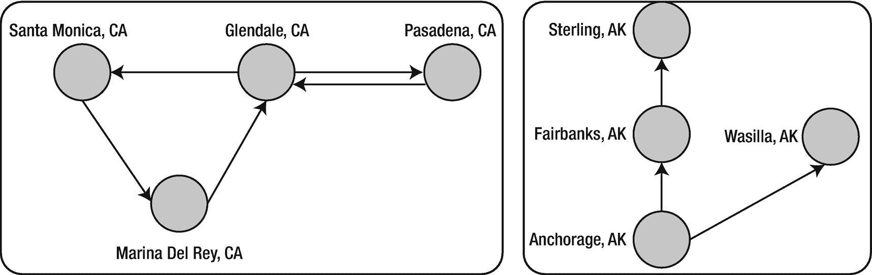
图 6-6

连接的组件

val vertices = Array((1L, ("Santa Monica","CA")),(2L,("Marina Del Rey","CA")),(3L, ("Glendale","CA")),(4L, ("Pasadena","CA")),(5L, ("Anchorage","AK")),(6L, ("Fairbanks","AK")),(7L, ("Sterling","AK")),(8L, ("Wasilla","AK")))

val vRDD = sc.parallelize(vertices)

val edges = Array(Edge(1L,2L,5),Edge(1L,3L,24),Edge(2L,3L,28),Edge(3L,4L,9),Edge(4L,3L,9),Edge(5L,6L,32),Edge(6L,7L,28),Edge(5L,8L,17))

val eRDD = sc.parallelize(edges)

val graph = Graph(vRDD,eRDD)

graph.vertices.collect.foreach(println)

(6,(Fairbanks,AK))
(3,(Glendale,CA))
(4,(Pasadena,CA))
(1,(Santa Monica,CA))
(7,(Sterling,AK))
(8,(Wasilla,AK))
(5,(Anchorage,AK))
(2,(Marina Del Rey,CA))

graph.edges.collect.foreach(println)

Edge(1,2,5)
Edge(1,3,24)
Edge(2,3,28)
Edge(3,4,9)
Edge(4,3,9)
Edge(5,6,32)
Edge(5,8,17)
Edge(6,7,28)

val connectedComponents = graph.connectedComponents()

connectedComponents.vertices.collect.foreach(println)

(6,5)
(3,1)
(4,1)
(1,1)
(7,5)
(8,5)
(5,5)
(2,1)

Listing 6-2Determine the Connected Components

图框架

GraphFrames 是一个建立在 DataFrames 之上的图处理库。在撰写本文时，GraphFrames 仍在积极开发中，但它成为核心 Apache Spark 框架的一部分只是时间问题。有几件事让 GraphFrames 比 GraphX 更强大。所有 GraphFrames 算法在 Java、Python 和 Scala 中都可用。可以使用熟悉的 DataFrames API 和 Spark SQL 来访问 GraphFrames。它还完全支持 DataFrame 数据源，允许使用几种支持的格式和数据源(如关系数据源、CSV、JSON 和 Parquet)来读取和写入图。 ^xiv 清单 6-3 展示了一个如何使用 GraphFrames 的例子。 ^xv

spark-shell --packages graphframes:graphframes:0.7.0-spark2.4-s_2.11

import org.graphframes._

val vDF = spark.createDataFrame(Array((1L, "Santa Monica","CA"),(2L,"Marina Del Rey","CA"),(3L, "Glendale","CA"),(4L, "Pasadena","CA"),(5L, "Anchorage","AK"),(6L, "Fairbanks","AK"),(7L, "Sterling","AK"),(8L, "Wasilla","AK"))).toDF("id","city","state")

vDF.show
+---+--------------+-----+
| id|          city|state|
+---+--------------+-----+
|  1|  Santa Monica|   CA|
|  2|Marina Del Rey|   CA|
|  3|      Glendale|   CA|
|  4|      Pasadena|   CA|
|  5|     Anchorage|   AK|
|  6|     Fairbanks|   AK|
|  7|      Sterling|   AK|
|  8|       Wasilla|   AK|
+---+--------------+-----+

val eDF = spark.createDataFrame(Array((1L,2L,5),(1L,3L,24),(2L,3L,28),(3L,4L,9),(4L,3L,9),(5L,6L,32),(6L,7L,28),(5L,8L,17))).toDF("src","dst","distance")

eDF.show
+---+----+--------+
|src|dest|distance|
+---+----+--------+
|  1|   2|       5|
|  1|   3|      24|
|  2|   3|      28|
|  3|   4|       9|
|  4|   3|       9|
|  5|   6|      32|
|  6|   7|      28|
|  5|   8|      17|
+---+----+--------+

val graph = GraphFrame(vDF,eDF)

graph.vertices.show
+---+--------------+-----+
| id|          city|state|
+---+--------------+-----+
|  1|  Santa Monica|   CA|
|  2|Marina Del Rey|   CA|
|  3|      Glendale|   CA|
|  4|      Pasadena|   CA|
|  5|     Anchorage|   AK|
|  6|     Fairbanks|   AK|
|  7|      Sterling|   AK|
|  8|       Wasilla|   AK|
+---+--------------+-----+

graph.edges.show

+---+---+--------+
|src|dst|distance|
+---+---+--------+
|  1|  2|       5|
|  1|  3|      24|
|  2|  3|      28|
|  3|  4|       9|
|  4|  3|       9|
|  5|  6|      32|
|  6|  7|      28|
|  5|  8|      17|
+---+---+--------+

graph.triplets.show

+--------------------+----------+--------------------+
|                 src|      edge|                 dst|
+--------------------+----------+--------------------+
|[1, Santa Monica,...|[1, 3, 24]|   [3, Glendale, CA]|
|[1, Santa Monica,...| [1, 2, 5]|[2, Marina Del Re...|
|[2, Marina Del Re...|[2, 3, 28]|   [3, Glendale, CA]|
|   [3, Glendale, CA]| [3, 4, 9]|   [4, Pasadena, CA]|
|   [4, Pasadena, CA]| [4, 3, 9]|   [3, Glendale, CA]|
|  [5, Anchorage, AK]|[5, 8, 17]|    [8, Wasilla, AK]|
|  [5, Anchorage, AK]|[5, 6, 32]|  [6, Fairbanks, AK]|
|  [6, Fairbanks, AK]|[6, 7, 28]|   [7, Sterling, AK]|
+--------------------+----------+--------------------+

graph.inDegrees.show

+---+--------+
| id|inDegree|
+---+--------+
|  7|       1|
|  6|       1|
|  3|       3|
|  8|       1|
|  2|       1|
|  4|       1|
+---+--------+

graph.outDegrees.show

+---+---------+
| id|outDegree|
+---+---------+
|  6|        1|
|  5|        2|
|  1|        2|
|  3|        1|
|  2|        1|
|  4|        1|
+---+---------+

sc.setCheckpointDir("/tmp")

val connectedComponents = graph.connectedComponents.run

connectedComponents.show

 +---+--------------+-----+---------+
| id|          city|state|component|
+---+--------------+-----+---------+
|  1|  Santa Monica|   CA|        1|
|  2|Marina Del Rey|   CA|        1|
|  3|      Glendale|   CA|        1|
|  4|      Pasadena|   CA|        1|
|  5|     Anchorage|   AK|        5|
|  6|     Fairbanks|   AK|        5|
|  7|      Sterling|   AK|        5|
|  8|       Wasilla|   AK|        5|
+---+--------------+-----+---------+

Listing 6-3GraphFrames Example

摘要

本章介绍使用 GraphX 和 GraphFrames 进行图分析。图分析是一个令人兴奋的快速发展的研究领域，具有广泛而深远的应用。我们只是触及了 GraphX 和 GraphFrames 的皮毛。虽然它可能不适合每个用例，但图分析对于它的设计用途来说是很棒的，并且是您的分析工具集不可或缺的一部分。

参考

1. 迈克尔·西蒙斯；《白手起家的亿万富翁查理·芒格有哪些与众不同的做法》，inc.com，2019， www.inc.com/michael-simmons/what-self-made-billionaire-charlie-munger-does-differently.html

2. 卡罗尔·麦克唐纳；《如何在 Scala 上使用 Apache Spark GraphX 入门》，mapr.com，2015， https://mapr.com/blog/how-get-started-using-apache-spark-graphx-scala/

3. 英伟达；“图分析”，开发者。英伟达。com ，2019， https://developer.nvidia.com/discover/graph-analytics

4. MathWorks《有向和无向图》，mathworks.com，2019， www.mathworks.com/help/matlab/math/directed-and-undirected-graphs.html

5. Rishi Yadav“第十一章，使用 GraphX 和 GraphFrames 进行图处理”，Packt Publishing，2017，Apache Spark 2.x Cookbook

6. 沃克·罗；“图数据库的用例”，bmc.com，2019， www.bmc.com/blogs/graph-database-use-cases/

7. 罗布·佩里；“数据传承:GDPR 全面合规的关键”，insidebigdata.com，2018， https://insidebigdata.com/2018/01/29/data-lineage-key-total-gdpr-compliance/

8. Avery Ching 等人；《一万亿条边:脸书尺度的图处理》，research.fb.com，2015， https://research.fb.com/publications/one-trillion-edges-graph-processing-at-facebook-scale/

9. 穆罕默德·古勒；“使用 Spark 进行图处理”，Apress，2015，使用 Spark 进行大数据分析

10. 火花；《房产图》，spark.apache.org，2015， https://spark.apache.org/docs/latest/graphx-programming-guide.html#the-property-graph

11. 火花；《示例属性图》，spark.apache.org，2019， https://spark.apache.org/docs/latest/graphx-programming-guide.html#the-property-graph

12. 火花；《地图减少三胞胎过渡指南》，spark.apache.org，2019， https://spark.apache.org/docs/latest/graphx-programming-guide.html#the-property-graph

13. 卡罗尔·麦克唐纳；《如何在 Scala 上使用 Apache Spark GraphX 入门》，mapr.com，2015， https://mapr.com/blog/how-get-started-using-apache-spark-graphx-scala/

14. 安库尔·戴夫等人；《GraphFrames 简介》，Databricks.com，2016， https://databricks.com/blog/2016/03/03/introducing-graphframes.html

15. Rishi Yadav“第十一章，使用 GraphX 和 GraphFrames 进行图处理”，Packt Publishing，2017，Apache Spark 2.x Cookbook

七、深度学习

明斯基和帕佩特如果能找到解决这个问题的方法，而不是把感知机打死，他们会做出更大的贡献。

—弗朗西斯·克里克 ^一世

深度学习是机器学习和人工智能的一个子领域，它使用深度、多层人工神经网络(图 7-1 )。由于它能够非常精确地执行类似人类的任务，所以最近非常流行。深度学习领域的进步已经在计算机视觉、语音识别、游戏和异常检测等领域开辟了令人兴奋的可能性。GPU(图形处理器)的主流可用性几乎在一夜之间推动了人工智能在全球的采用。高性能计算已经变得足够强大，以至于仅仅几年前在计算上似乎不可能的任务现在都可以在多 GPU 云实例或廉价机器集群上例行执行。这使得人工智能领域的众多创新以过去不可能的速度发展。

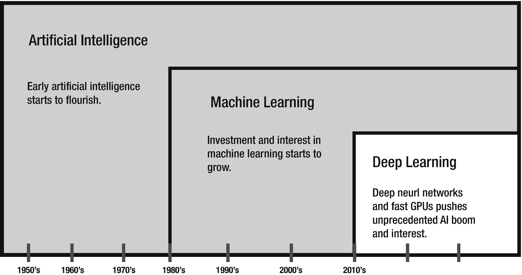
图 7-1

AI、机器学习、深度学习的关系 ⁱⁱ

深度学习是人工智能领域最近许多突破的原因。虽然深度学习可以用于更平凡的分类任务，但当应用于更复杂的问题时，如医疗诊断、面部识别、自动驾驶汽车、欺诈分析和智能语音控制助理，它的真正力量会大放异彩。 ⁱⁱⁱ 在某些领域，深度学习已经使计算机能够匹配甚至超越人类的能力。例如，通过深度学习，谷歌 DeepMind 的 AlphaGo 程序能够在围棋中击败韩国大师李世石，这是有史以来最复杂的棋盘游戏之一。围棋比国际象棋等其他棋类游戏复杂得多。它有 10 的 170 次方个可能的板配置，这比宇宙中的原子数量还要多。 ^iv 另一个很好的例子是特斯拉。特斯拉使用深度学习 ^v 来为其自动驾驶功能提供动力，处理来自其制造的每辆汽车中内置的几个环绕摄像头、超声波传感器和前向雷达的数据。为了向其深度神经网络提供高性能处理能力，特斯拉为其自动驾驶汽车配备了一台使用自己的人工智能芯片的计算机，配备了 GPU、CPU 和深度学习加速器，每秒可进行 144 万亿次运算(TOPS)。 ^vi

与其他机器学习算法类似，深度神经网络通常在更多的训练数据下表现更好。这就是火花出现的原因。但是，尽管 Spark MLlib 包括一系列广泛的机器学习算法，但在撰写本文时，其深度学习支持仍然有限(Spark MLlib 包括一个多层感知器分类器，一个完全连接的前馈神经网络，仅限于训练浅层网络和执行迁移学习)。然而，由于谷歌和脸书等开发商和公司的社区，有几个第三方分布式深度学习库和框架与 Spark 集成。我们将探索一些最受欢迎的。在这一章中，我将关注最流行的深度学习框架之一:Keras。对于分布式深度学习，我们将使用 Elephas 和分布式 Keras (Dist-Keras)。我们将在本章通篇使用 Python。我们将使用 PySpark 作为我们的分布式深度学习示例。

神经网络

神经网络是一类算法，其操作类似于人脑的互连神经元。神经网络包含由互连节点组成的多层。通常有一个输入层，一个或多个隐藏层，一个输出层(图 7-2 )。数据经由输入层通过神经网络。隐藏层通过加权连接网络处理数据。隐藏层中的节点为输入分配权重，并将其与一组系数组合。数据通过一个节点的激活函数，该函数决定了层的输出。最后，数据到达输出层，输出层产生神经网络的最终输出。VII

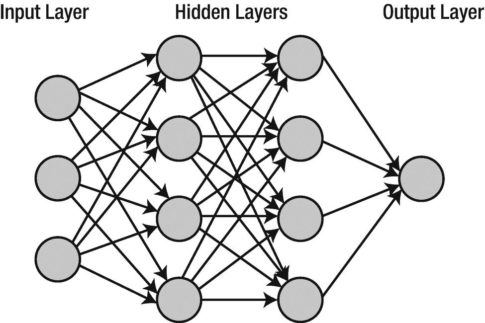
图 7-2

一个简单的神经网络

具有几个隐藏层的神经网络被称为“深度”神经网络。层次越多，网络就越深，通常网络越深，学习就变得越复杂，它能解决的问题也越复杂。这就是赋予深度神经网络达到最先进精度的能力。有几种类型的神经网络:前馈神经网络、循环神经网络和自动编码器神经网络，每种神经网络都有自己的功能，并为不同的目的而设计。前馈神经网络或多层感知器适用于结构化数据。对于音频、时间序列或文本等序列数据，循环神经网络是一个很好的选择。 ^viii 自动编码器是异常检测和降维的好选择。一种类型的神经网络，卷积神经网络，由于其在计算机视觉领域的革命性性能，最近在世界上掀起了风暴。

神经网络简史

第一个神经网络，麦卡洛克-皮茨神经元，是由沃伦·麦卡洛克和沃尔特·皮茨在 1943 年开发的，并在他们的开创性论文“神经活动内在思想的逻辑演算”中进行了描述 ^ix 麦卡洛克-皮茨神经元并不像现代的神经网络，但它是为我们今天所知的人工智能的诞生铺平道路的种子。弗兰克·罗森布拉特于 1958 年推出的感知机是神经网络领域的下一个革命性发展。Rosenblatt 感知器是一个简单的单层神经网络，用于二进制分类。它是在康奈尔航空实验室构思的，最初是用 IBM 704 用软件模拟的。罗森布拉特的工作最终创造了 Mark I 感知器，这是一种为图像识别而定制的机器。20 世纪 60 年代末，在马文·明斯基和西蒙·派珀特出版了《?? 感知器》之后，人们对感知器的兴趣开始减弱，这本极具影响力的书阐述了感知器的局限性，尤其是它无法学习非线性函数。明斯基和帕佩特对联结主义模型的过分热情和有时充满敌意(多年后他们承认了这一点)的批判导致了 20 世纪 80 年代人工智能研究的兴趣和资金减少。这种情况进一步加剧，部分原因是支持向量机(SVM)和图形模型的成功，以及符号人工智能(从 20 世纪 50 年代到 80 年代末流行的人工智能范式)的日益流行。尽管如此，许多科学家和研究人员，如吉姆·安德森、大卫·威尔肖和斯蒂芬·格罗斯伯格，仍然默默地继续着他们对神经网络的研究。1975 年，Kunihiko Fukushima 在日本东京 Segataya 的 NHK 科学技术研究实验室担任研究科学家，开发了第一个多层神经网络 neocognitron。 ^十三

神经网络在 20 世纪 80 年代中期再次兴起，在此期间，许多先驱发明了许多对现代深度学习至关重要的基本概念和技术。1986 年，Geoffrey Hinton(被许多人视为“人工智能教父”)推广了反向传播，这是神经网络学习的基本方法，也是几乎所有现代神经网络实现的核心。 ^xiv 同样重要的是，Hinton 和他的团队推广了使用多层神经网络学习非线性函数的想法，直接解决了 Minsky 和 Papert 在感知器中的批评。辛顿的工作有助于将神经网络从默默无闻中带回到聚光灯下。Yann LeCun 受福岛新认知神经的启发，在 20 世纪 80 年代末开发了卷积神经网络。1988 年在贝尔实验室时，Yann LeCun 使用卷积神经网络来识别手写字符。美国电话电报公司将该系统出售给银行，以读取和识别支票上的笔迹，并被认为是神经网络的第一个现实应用。^XVIyo shua beng io 因其引入了单词嵌入的概念以及最近与 Ian Goodfellow 合作研究生成对抗网络(GANs)而闻名，生成对抗网络是一种深度神经网络架构，由两个彼此对立或“对抗”的神经网络组成。Yann LeCun 将对抗性训练描述为“过去 10 年机器学习中最有趣的想法。” ^xvii 三位先驱最近获得了 2018 年的图灵奖。

尽管如此，尽管有这些创新，但神经网络的实际应用仍然不是每个人都能达到的，而是最大的公司和资金充足的大学，因为需要大量的计算资源来训练它们。正是经济实惠的高性能 GPU 的广泛使用将神经网络推向了主流。以前被认为是不可扩展和不切实际的训练，神经网络突然开始在计算机视觉、语音识别、游戏和其他历史上困难的机器学习任务领域提供类似人类的性能，使用 GPU 具有非凡的准确性。当 Alex Krizhevsky、Ilya Sutskever 和 Geoff Hinton 开发的经过 GPU 训练的卷积神经网络 AlexNet 在 2012 年赢得 ImageNet 大规模视觉识别比赛时，世界受到了关注。 ^xviii 它以如此大的优势赢得了比赛，比亚军低了 10.8 个百分点，前五名的误差为 15.3%。 ^xix AlexNet 还普及了现在在大多数 CNN 架构中常见的大部分原则，如使用整流线性单元(ReLU)激活功能，使用辍学和数据增强来减少过拟合，重叠池，以及在多个 GPU 上训练。

最近，学术界和私营部门在人工智能领域都有前所未有的创新。谷歌、亚马逊、微软、脸书、IBM、特斯拉、英伟达等公司正在深度学习领域投入大量资源，进一步拓展人工智能的边界。斯坦福大学、卡内基梅隆大学和麻省理工学院等领先大学以及 OpenAI 和艾伦人工智能研究所等研究机构正在以惊人的速度发表突破性的研究。从全球来看，令人印象深刻的创新来自中国、加拿大、英国和澳大利亚等国家。

卷积神经网络

卷积神经网络(简称为 convnet 或 CNN)是一种特别擅长分析图像的神经网络(尽管它们也可以应用于音频和文本数据)。卷积神经网络层中的神经元以三维方式排列:高度、宽度和深度。CNN 使用卷积层来学习其输入特征空间(图像)中的局部模式，例如纹理和边缘。相反，全连接(密集)层学习全局模式。 ^xx 卷积层中的神经元仅连接到其之前层的一小部分区域，而不是像密集层那样连接到所有神经元。密集层的完全连接结构会导致大量的参数，这是低效的，并可能很快导致过度拟合。XXI

在我们继续讨论卷积神经网络之前，理解颜色模型的概念是很重要的。图像被表示为像素的集合。 ^xxii 像素是构成图像的最小信息单位。灰度图像的像素值范围从 0(黑色)到 255(白色)，如图 7-3 (a)所示。灰度图像只有一个通道。RGB 是最传统的颜色模型。RGB 图像有三个通道:红色、绿色和蓝色。这意味着 RGB 图像中的每个像素由三个 8 位数字表示(图 7-3 (b))，每个数字的范围从 0 到 255。使用这些通道的不同组合会显示不同的颜色。

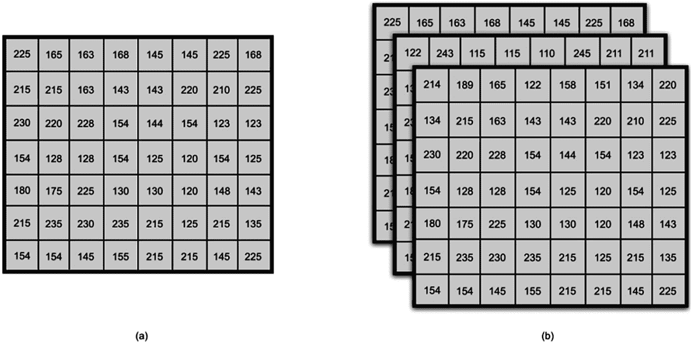
图 7-3

灰度和 RGB 图像

卷积神经网络接受形状的三维张量作为输入:图像的高度、重量和深度(图 7-4 )。图像的深度是通道的数量。对于灰度图像，深度为 1，而对于 RGB 图像，深度为 3。在图 7-4 中，图像的输入形状为(7，8，3)。

图 7-4

单个图像的输入形状

卷积神经网络体系结构

图 7-5 显示了典型的 CNN 架构的样子。卷积神经网络由几层组成，每层都试图识别和学习各种特征。层的主要类型是卷积层、汇集层和全连接层。这些层可以进一步分为两个主要类别:特征检测层和分类层。

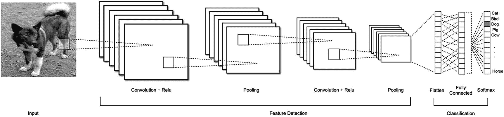
图 7-5

一种用于分类动物图像的 CNN 架构^XXIII

特征检测图层

卷积层

卷积层是卷积神经网络的主要构件。卷积层使输入图像通过一系列激活输入图像的某些特征的卷积核或滤波器。卷积是一种数学运算，当内核在输入特征地图上滑动(或跨越)时，在输入元素和内核元素重叠的每个位置执行逐元素乘法。将结果相加以产生当前位置的输出。对每一步重复该过程，生成称为输出特征地图的最终结果。XXIV图 7-6 展示了一个 3×3 的卷积核。图 7-7 显示了一个 2D 卷积，其中我们的 3 x 3 内核被应用于一个 5 x 5 输入特征映射，产生一个 3 x 3 输出特征映射。我们使用步长 1，这意味着内核从当前位置移动一个像素到下一个像素。

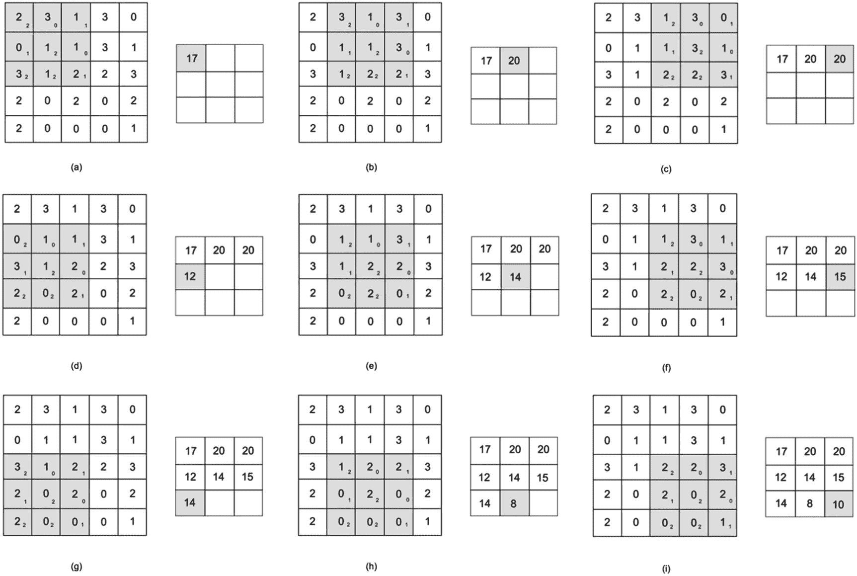
图 7-7

一种 2D 卷积，其中将 3 x 3 内核应用于 5 x 5 输入要素地图(25 个要素)，从而生成一个包含 9 个输出要素的 3 x 3 输出要素地图

图 7-6

3×3 卷积核

对于 RGB 图像，3D 卷积涉及每个输入通道的一个核(总共 3 个核)。所有结果相加形成一个输出。添加用于帮助激活函数更好地拟合数据的偏差项，以创建最终的输出特征图。

整流线性单元(ReLU)激活功能

通常的做法是在每个卷积层之后包括一个激活层。激活函数也可以通过所有转发层支持的激活参数来指定。激活函数将节点的输入转换成输出信号，该输出信号用作下一层的输入。激活功能通过允许神经网络学习更复杂的数据，如图像、音频和文本，使神经网络更强大。它通过向我们的神经网络引入非线性特性来做到这一点。如果没有激活函数，神经网络将只是一个过于复杂的线性回归模型，只能处理简单的线性问题。 ^xxv Sigmoid 和 tanh 也是常见的激活层。整流线性单元(ReLU)是大多数 CNN 最流行和首选的激活功能。ReLU 返回它收到的任何实际输入的值，但如果收到负值，则返回 0。已经发现 ReLU 有助于加速模型训练，而不会显著影响准确性。

汇集层

池图层通过缩小输入影像的维度来降低计算复杂度和参数数量。通过减少维度，池层也有助于控制过度拟合。在每个卷积层之后插入一个汇集层也是很常见的。有两种主要的池:平均池和最大池。平均池使用来自每个池区域的所有值的平均值(图 7-8 (b))，而最大池使用最大值(图 7-8 (a))。在某些架构中，使用更大的跨度比使用池层更可取。

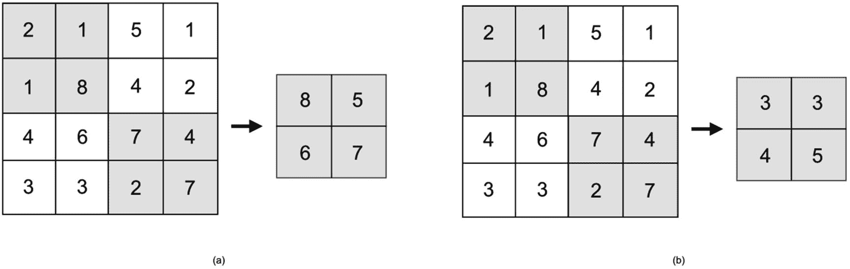
图 7-8

最大和平均池

分类层

展平图层

在将数据馈送到完全连接的密集图层之前，展平图层会将二维矩阵转换为一维向量。

全连接(密集)层

完全连接的图层(也称为密集图层)接收来自平整图层的数据，并输出包含每个类概率的矢量。

脱落层

在训练期间，一个脱落层随机地去激活网络中的一些神经元。丢弃是一种正则化形式，有助于降低模型复杂性并防止过度拟合。

Softmax 和 Sigmoid 函数

最终的密集层提供分类输出。它将 softmax 函数用于多类分类任务，或者将 sigmoid 函数用于二元分类任务。

深度学习框架

本节提供了当前可用的一些最流行的深度学习框架的快速概述。这绝不是一份详尽的清单。这些框架中的大多数或多或少都有相同的特性。它们在社区和行业采用程度、受欢迎程度和生态系统规模方面有所不同。

TensorFlow

TensorFlow 是目前最流行的深度学习框架。它是谷歌开发的，作为 Theano 的替代品。Theano 最初的一些开发者去了 Google，开发了 TensorFlow。TensorFlow 提供了一个运行在用 C/C++开发的引擎之上的 Python API。

提亚诺

Theano 是最早的开源深度学习框架之一。它最初由蒙特利尔大学的蒙特利尔学习算法研究所(MILA)于 2007 年发布。2017 年 9 月，Yoshua Bengio 正式宣布将结束对 Theano 的开发。^XXVI

PyTorch

PyTorch 是由脸书人工智能研究(FAIR)小组开发的开源深度学习库。PyTorch 用户采用率最近一直在飙升，是第三大最受欢迎的框架，仅次于 TensorFlow 和 Keras。

深度学习 4J

DeepLearning4J 是一个用 Java 编写的深度学习库。它与 Scala 等基于 JVM 的语言兼容，并与 Spark 和 Hadoop 集成。它使用自己的开源科学计算库 ND4J，而不是 Breeze。对于更喜欢 Java 或 Scala 而不是 Python 进行深度学习的开发人员来说，DeepLearning4J 是一个很好的选择(尽管 DeepLearning4J 有一个使用 Keras 的 Python API)。

CNT(消歧义)

CNTK 又称微软认知工具包，是微软研究院开发的深度学习库，于 2015 年 4 月开源。它使用一系列计算步骤，使用有向图来描述神经网络。CNTK 支持跨多个 GPU 和服务器的分布式深度学习。

硬

Keras 是由 Francois Chollet 在谷歌开发的高级深度学习框架。它提供了一个简单的模块化 API，可以运行在 TensorFlow、Theano 和 CNTK 之上。它享有广泛的行业和社区采用和充满活力的生态系统。Keras 模型可以部署在 iOS 和 Android 设备上，通过 Keras.js 和 WebDNN 部署在浏览器中，部署在 Google Cloud 上，通过 Skymind 的 DL4J 导入功能部署在 JVM 上，甚至部署在 Raspberry Pi 上。Keras 开发主要由谷歌支持，但微软、亚马逊、英伟达、优步和苹果也是主要的项目贡献者。像其他框架一样，它具有出色的多 GPU 支持。对于最复杂的深度神经网络，Keras 通过 Horovod、Google Cloud 上的 GPU 集群以及 Dist-Keras 和 Elephas 上的 Spark 支持分布式训练。

使用 Keras 进行深度学习

我们将使用 Keras Python API 和 TensorFlow 作为所有深度学习示例的后端。我们将在本章后面的分布式深度学习示例中使用 PySpark 和 Elephas 以及分布式 Keras。

使用 Iris 数据集的多类分类

我们将使用一个熟悉的数据集进行我们的第一个神经网络分类 ^xxvii 任务(列表 7-1 )。如前所述，我们将在本章的所有例子中使用 Python。

import numpy as np

from keras.models import Sequential
from keras.optimizers import Adam
from keras.layers import Dense

from sklearn.model_selection import train_test_split
from sklearn.preprocessing import OneHotEncoder
from sklearn.datasets import load_iris

# Load the Iris dataset.
iris_data = load_iris()

x = iris_data.data

# Inspect the data. We'll truncate
# the output for brevity.

print(x)
[[5.1 3.5 1.4 0.2]
 [4.9 3\.  1.4 0.2]
 [4.7 3.2 1.3 0.2]
 [4.6 3.1 1.5 0.2]
 [5\.  3.6 1.4 0.2]
 [5.4 3.9 1.7 0.4]
 [4.6 3.4 1.4 0.3]
 [5\.  3.4 1.5 0.2]
 [4.4 2.9 1.4 0.2]
 [4.9 3.1 1.5 0.1]]

# Convert the class label into a single column.
y = iris_data.target.reshape(-1, 1)

# Inspect the class labels. We'll truncate
# the output for brevity.

print(y)
[[0]
 [0]
 [0]
 [0]
 [0]
 [0]
 [0]
 [0]
 [0]
 [0]]

# It's considered best practice to one-hot encode the class labels
# when using neural networks for multiclass classification tasks.

encoder = OneHotEncoder(sparse=False)
enc_y = encoder.fit_transform(y)
print(enc_y)

[[1\. 0\. 0.]
 [1\. 0\. 0.]
 [1\. 0\. 0.]
 [1\. 0\. 0.]
 [1\. 0\. 0.]
 [1\. 0\. 0.]
 [1\. 0\. 0.]
 [1\. 0\. 0.]
 [1\. 0\. 0.]
 [1\. 0\. 0.]]

# Split the data for training and testing.
# 70% for training dataset, 30% for test dataset.

train_x, test_x, train_y, test_y = train_test_split(x, enc_y, test_size=0.30)

# Define the model.

# We instantiate a Sequential model consisting of a linear stack of layers.
# Since we are dealing with a one-dimensional feature vector, we will use
# dense layers in our network. We use convolutional layers later in the
# chapter when working with images.

# We use ReLU as the activation function on our fully connected layers.
# We can name any layer by passing the name argument. We pass the number
# of features to the input_shape argument, which is 4 (petal_length,
# petal_width, sepal_length, sepal_width)

model = Sequential()
model.add(Dense(10, input_shape=(4,), activation="relu", name="fclayer1"))
model.add(Dense(10, activation="relu", name="fclayer2"))

# We use softmax activation function in our output layer. As discussed,
# using softmax activation layer allows the model to perform multiclass
# classification. For binary classification, use the sigmoid activation
# function instead. We specify the number of class, which in our case is 3.

model.add(Dense(3, activation="softmax", name="output"))

# Compile the model. We use categorical_crossentropy for multiclass
# classification. For binary classification, use binary_crossentropy.

model.compile(loss='categorical_crossentropy', optimizer="adam", metrics=['accuracy'])

# Display the model summary.

print(model.summary())

Model: "sequential_1"
_________________________________________________________________
Layer (type)                 Output Shape              Param #
=================================================================
fclayer1 (Dense)             (None, 10)                50
_________________________________________________________________
fclayer2 (Dense)             (None, 10)                110
_________________________________________________________________
output (Dense)               (None, 3)                 33
=================================================================
Total params: 193
Trainable params: 193
Non-trainable params: 0
_________________________________________________________________
None

# Train the model on training dataset with epochs set to 100
# and batch size to 5\. The output is edited for brevity.

model.fit(train_x, train_y, verbose=2, batch_size=5, epochs=100)
Epoch 1/100
 - 2s - loss: 1.3349 - acc: 0.3333
Epoch 2/100
 - 0s - loss: 1.1220 - acc: 0.2952
Epoch 3/100
 - 0s - loss: 1.0706 - acc: 0.3429
Epoch 4/100
 - 0s - loss: 1.0511 - acc: 0.3810
Epoch 5/100
 - 0s - loss: 1.0353 - acc: 0.3810
Epoch 6/100
 - 0s - loss: 1.0175 - acc: 0.3810
Epoch 7/100
 - 0s - loss: 1.0013 - acc: 0.4000
Epoch 8/100
 - 0s - loss: 0.9807 - acc: 0.4857
Epoch 9/100
 - 0s - loss: 0.9614 - acc: 0.6667
Epoch 10/100
 - 0s - loss: 0.9322 - acc: 0.6857
...
Epoch 97/100
 - 0s - loss: 0.1510 - acc: 0.9524
Epoch 98/100
 - 0s - loss: 0.1461 - acc: 0.9810
Epoch 99/100
 - 0s - loss: 0.1423 - acc: 0.9810
Epoch 100/100
 - 0s - loss: 0.1447 - acc: 0.9810
<keras.callbacks.History object at 0x7fbb93a50510>

# Test on test dataset.
results = model.evaluate(test_x, test_y)
45/45 [==============================] - 0s 586us/step

print('Accuracy: {:4f}'.format(results[1]))
Accuracy: 0.933333

Listing 7-1Multiclass Classification with Keras Using the Iris Dataset

那很有趣。然而，当用于涉及图像等非结构化数据的更复杂问题时，神经网络确实大放异彩。对于我们的下一个例子，我们将使用卷积神经网络来执行手写数字识别。

用 MNIST 识别手写数字

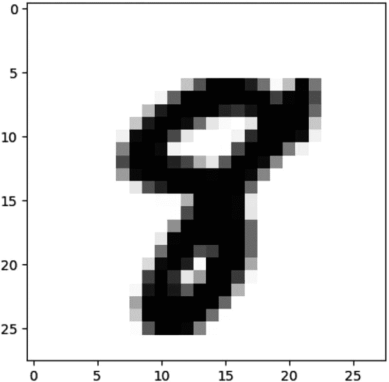
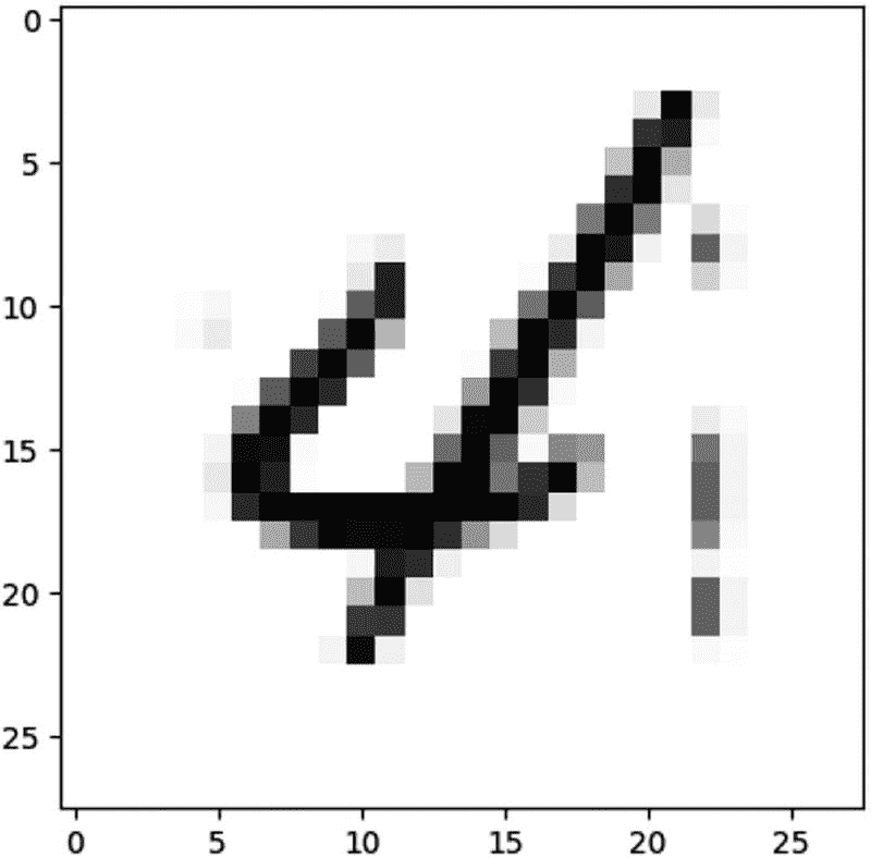
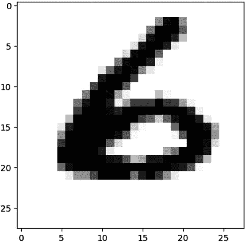
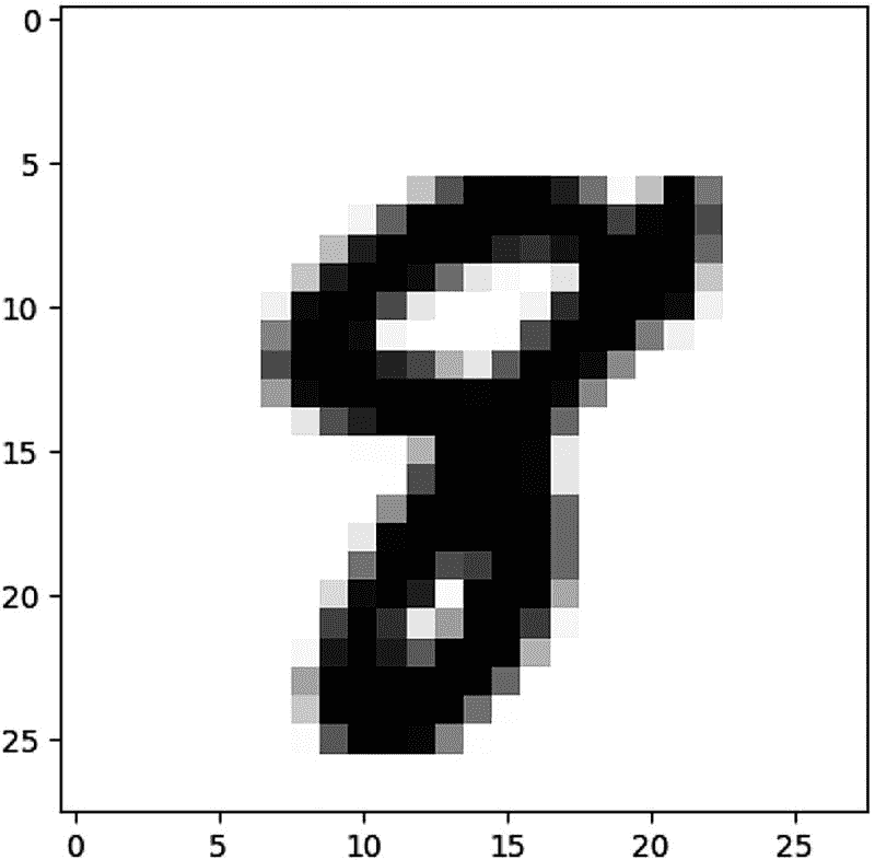
MNIST 数据集是来自美国国家标准和技术研究所(NIST)的手写数字图像的数据库。该数据集包含 70，000 幅图像:60，000 幅图像用于训练，10，000 幅图像用于测试。都是 0 到 9 的 28 x 28 灰度图像(图 7-9 )。见清单 7-2 。

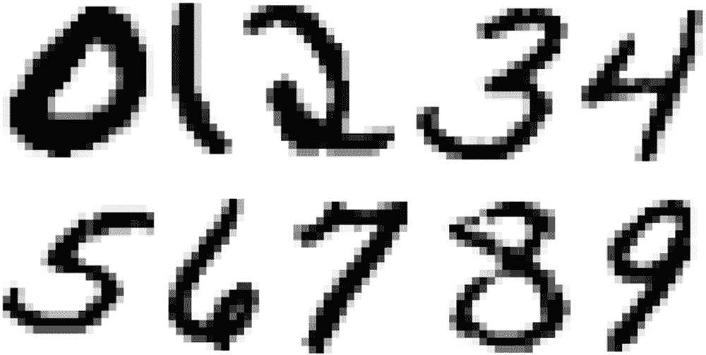
图 7-9

来自 MNIST 手写数字数据库的样本图像

import keras
import matplotlib.pyplot as plt

from keras.datasets import mnist
from keras.models import Sequential
from keras.layers import Dense, Conv2D, Dropout, Flatten, MaxPooling2D

# Download MNIST data.

(x_train, y_train), (x_test, y_test) = mnist.load_data()

image_idx = 400
print(y_train[image_idx])

# Inspect the data.

2

plt.imshow(x_train[image_idx], cmap="Greys")
plt.show()

Listing 7-2Handwritten Digit Recognition with MNIST Using Keras

# Check another number.

image_idx = 600
print(y_train[image_idx])
9

plt.imshow(x_train[image_idx], cmap="Greys")
plt.show()

# Get the "shape" of the dataset.
x_train.shape
(60000, 28, 28)

# Let’s reshape the array to 4-dims so that it can work with Keras.
# The images are 28 x 28 grayscale. The last parameter, 1, indicates
# that images are grayscale. For RGB, set the parameter to 3.

x_train = x_train.reshape(x_train.shape[0], 28, 28, 1)
x_test = x_test.reshape(x_test.shape[0], 28, 28, 1)

# Convert the values to float before division.

x_train = x_train.astype('float32')
x_test = x_test.astype('float32')

# Normalize the RGB codes.

x_train /= 255
x_test /= 255
print'x_train shape: ', x_train.shape
x_train shape:  60000, 28, 28, 1

print'No. of images in training dataset: ', x_train.shape[0]
No. of images in training dataset:  60000

print'No. of images in test dataset: ', x_test.shape[0]
No. of images in test dataset:  10000

# Convert class vectors to binary class matrices. We also pass
# the number of classes (10).

y_train = keras.utils.to_categorical(y_train, 10)
y_test = keras.utils.to_categorical(y_test, 10)

# Build the CNN. Create a Sequential model and add the layers.

model = Sequential()
model.add(Conv2D(28, kernel_size=(3,3), input_shape= (28,28,1), name="convlayer1"))

# Reduce the dimensionality using max pooling.

model.add(MaxPooling2D(pool_size=(2, 2)))

# Next we need to flatten the two-dimensional arrays into a one-dimensional feature vector. This will allow us to perform classification.

model.add(Flatten())
model.add(Dense(128, activation="relu",name='fclayer1'))

# Before we classify the data, we use a dropout layer to randomly
# deactivate some of the neurons. Dropout is a form of regularization
# used to help reduce model complexity and prevent overfitting.

model.add(Dropout(0.2))

# We add the final layer. The softmax layer (multinomial logistic
# regression) should have the total number of classes as parameter.
# In this case the number of parameters is the number of digits (0–9)
# which is 10.

model.add(Dense(10,activation='softmax', name="output"))

# Compile the model.

model.compile(optimizer='adam', loss="categorical_crossentropy", metrics=['accuracy'])

# Train the model.

model.fit(x_train,y_train,batch_size=128, verbose=1, epochs=20)

Epoch 1/20
60000/60000 [==============================] - 11s 180us/step - loss: 0.2742 - acc: 0.9195
Epoch 2/20
60000/60000 [==============================] - 9s 144us/step - loss: 0.1060 - acc: 0.9682
Epoch 3/20
60000/60000 [==============================] - 9s 143us/step - loss: 0.0731 - acc: 0.9781
Epoch 4/20
60000/60000 [==============================] - 9s 144us/step - loss: 0.0541 - acc: 0.9830
Epoch 5/20
60000/60000 [==============================] - 9s 143us/step - loss: 0.0409 - acc: 0.9877
Epoch 6/20
60000/60000 [==============================] - 9s 144us/step - loss: 0.0337 - acc: 0.9894
Epoch 7/20
60000/60000 [==============================] - 9s 143us/step - loss: 0.0279 - acc: 0.9910
Epoch 8/20
60000/60000 [==============================] - 9s 144us/step - loss: 0.0236 - acc: 0.9922
Epoch 9/20
60000/60000 [==============================] - 9s 143us/step - loss: 0.0200 - acc: 0.9935
Epoch 10/20
60000/60000 [==============================] - 9s 144us/step - loss: 0.0173 - acc: 0.9940
Epoch 11/20
60000/60000 [==============================] - 9s 143us/step - loss: 0.0163 - acc: 0.9945
Epoch 12/20
60000/60000 [==============================] - 9s 143us/step - loss: 0.0125 - acc: 0.9961
Epoch 13/20
60000/60000 [==============================] - 9s 143us/step - loss: 0.0129 - acc: 0.9956
Epoch 14/20
60000/60000 [==============================] - 9s 144us/step - loss: 0.0125 - acc: 0.9958
Epoch 15/20
60000/60000 [==============================] - 9s 144us/step - loss: 0.0102 - acc: 0.9968
Epoch 16/20
60000/60000 [==============================] - 9s 143us/step - loss: 0.0101 - acc: 0.9964
Epoch 17/20
60000/60000 [==============================] - 9s 143us/step - loss: 0.0096 - acc: 0.9969
Epoch 18/20
60000/60000 [==============================] - 9s 143us/step - loss: 0.0096 - acc: 0.9968
Epoch 19/20
60000/60000 [==============================] - 9s 142us/step - loss: 0.0090 - acc: 0.9972
Epoch 20/20
60000/60000 [==============================] - 9s 144us/step - loss: 0.0097 - acc: 0.9966

<keras.callbacks.History object at 0x7fc63d629850>

# Evaluate the model.

evalscore = model.evaluate(x_test, y_test, verbose=0)
print'Test accuracy: ', evalscore[1]
Test accuracy:  0.9851
print'Test loss: ', evalscore[0]
Test loss:  0.06053220131823819

# Let’s try recognizing some digits.

image_idx = 6700
plt.imshow(x_test[image_idx].reshape(28, 28),cmap='Greys')
plt.show()

pred = model.predict(x_test[image_idx].reshape(1, 28, 28, 1))
print(pred.argmax())
4

image_idx = 8200
plt.imshow(x_test[image_idx].reshape(28, 28),cmap='Greys')
plt.show()

pred = model.predict(x_test[image_idx].reshape(1, 28, 28, 1))
print(pred.argmax())
6

image_idx = 8735
plt.imshow(x_test[image_idx].reshape(28, 28),cmap='Greys')
plt.show()

pred = model.predict(x_test[image_idx].reshape(1, 28, 28, 1))
print(pred.argmax())
8

恭喜你！我们的模型能够准确地识别数字。

Spark 分布式深度学习

训练像多目标探测器这样的复杂模型可能需要几个小时、几天甚至几周的时间。在大多数情况下，单个多 GPU 机器足以在合理的时间内训练大型模型。对于要求更高的工作负载，将计算分散到多台机器上可以大大减少训练时间，实现快速迭代实验并加速深度学习部署。

Spark 的并行计算和大数据能力使其成为分布式深度学习的理想平台。使用 Spark 进行分布式深度学习有额外的好处，特别是如果您已经有一个现有的 Spark 集群。分析存储在同一个集群上的大量数据是很方便的，比如 HDFS、Hive、Impala 或 HBase。您可能还希望与同一集群中运行的其他类型的工作负载共享结果，例如商业智能、机器学习、ETL 和功能工程。^XXVIII

模型并行性与数据并行性

神经网络的分布式训练有两种主要方法:模型并行和数据并行。在数据并行中，分布式环境中的每个服务器都获得了模型的完整副本，但只是数据的一部分。训练在每个服务器中由完整数据集切片上的模型副本本地执行(图 7-10 (a))。在模型并行中，模型被分割在不同的服务器上(图 7-10 (b))。每个服务器被分配并负责处理单个神经网络的不同部分，例如层。 ^xxx 数据并行由于其简单性和易实现性，通常更受欢迎。但是，对于太大而无法在单台机器上安装的训练模型，模型并行是首选。Google 的大规模分布式深度学习框架 DistBelief 同时支持模型和数据并行。来自优步的分布式训练框架 Horovod 也支持模型和数据并行。

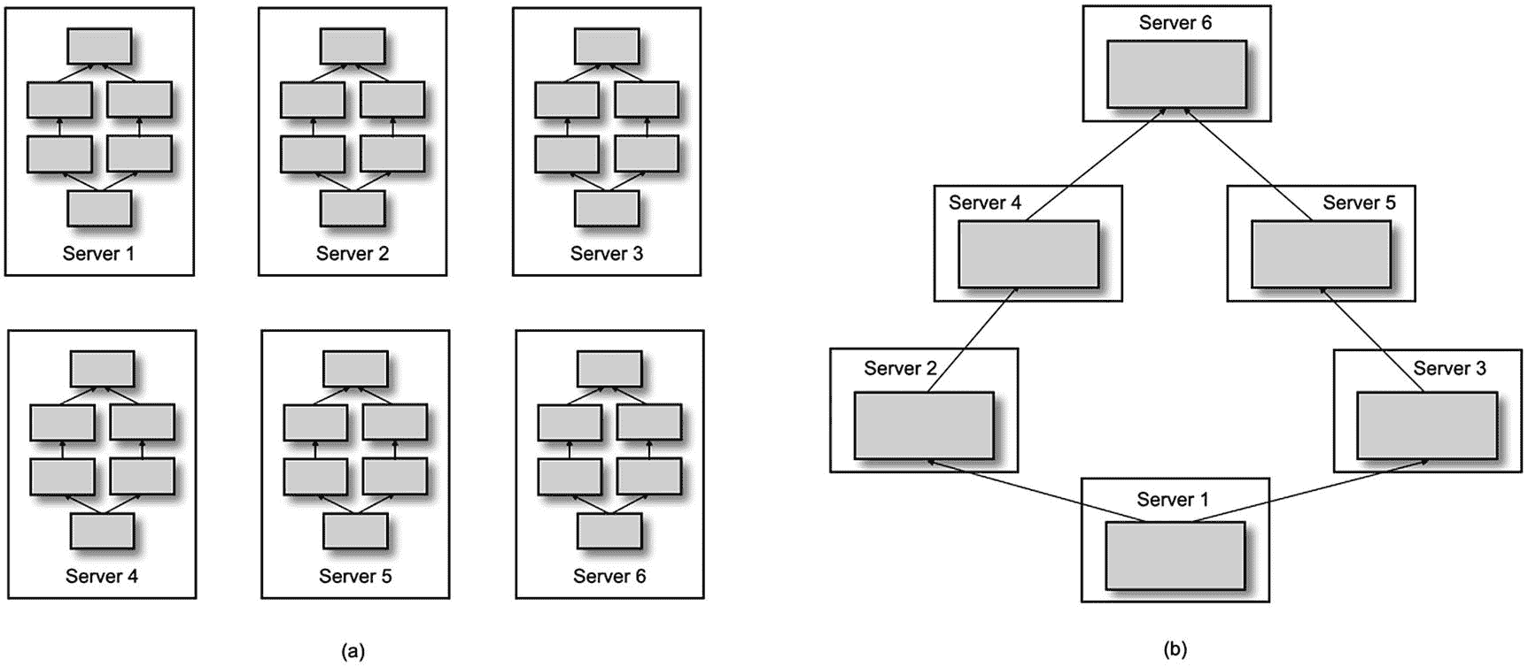
图 7-10

数据并行性与模型并行性 ^xxix

Spark 的分布式深度学习框架

感谢第三方贡献者，即使 Spark 的深度学习支持仍在开发中，也有几个外部分布式深度学习框架运行在 Spark 之上。我们将描述最受欢迎的。

深度学习管道

深度学习管道是来自 Databricks(由创建 Spark 的同一批人创建的公司)的第三方包，它提供了集成到 Spark ML 管道 API 中的深度学习功能。深度学习管道 API 使用 TensorFlow 和 Keras，TensorFlow 作为后端。它包括一个 ImageSchema，可用于将图像加载到 Spark 数据帧中。它支持迁移学习、分布式超参数调优以及将模型部署为 SQL 函数。在撰写本文时，深度学习管道仍在积极开发中。

BigDL

BigDL 是英特尔 Apache Spark 的分布式深度学习库。它与大多数深度学习框架的不同之处在于，它只支持 CPU。它使用多线程和英特尔的深度神经网络数学内核库(英特尔 MKL-DNN)，这是一个开源库，用于加速英特尔架构上深度学习框架的性能。据说性能可以与传统的 GPU 相媲美。

咖啡馆

CaffeOnSpark 是雅虎开发的深度学习框架。它是 Caffe 的分布式扩展，旨在 Spark 集群之上运行。雅虎广泛使用 CaffeOnSpark 进行内容分类和图片搜索。

TensorFlowOnSpark

TensorFlowOnSpark 是雅虎开发的另一个深度学习框架。它支持使用 Spark 的分布式张量流推理和训练。它与 Spark ML 管道集成，支持模型和数据并行以及异步和同步训练。

张量框架

TensorFrames 是一个实验库，允许 TensorFlow 轻松处理 Spark 数据帧。它支持 Scala 和 Python，并提供了在 Spark 和 TensorFlow 之间传递数据的有效方式，反之亦然。

他们是

Elephas 是一个 Python 库，它扩展了 Keras，以支持使用 Spark 进行高度可扩展的分布式深度学习。Elephas 由 Max Pumperla 开发，利用数据并行实现分布式深度学习，以易用性和简单性著称。它还支持分布式超参数优化和集合模型的分布式训练。

分布式 Keras

分布式 Keras (Dist-Keras)是另一个运行在 Keras 和 Spark 之上的分布式深度学习框架。它是由欧洲粒子物理研究所的游里·赫尔曼斯开发的。它支持多种分布式优化算法，如 ADAG、动态 SGD、异步弹性平均 SGD (AEASGD)、异步弹性平均动量 SGD (AEAMSGD)和倾盆大雨 SGD。

如前所述，这一章将集中讨论大象和分布式 Keras。

Elephas:使用 Keras 和 Spark 的分布式深度学习

Elephas 是一个 Python 库，它扩展了 Keras，以支持使用 Spark 进行高度可扩展的分布式深度学习。已经超越单个多 GPU 机器的 Keras 用户正在寻找无需重写现有 Keras 程序即可扩展模型训练的方法。Elephas(和分布式 Keras)提供了一种简单的方法来实现这一点。

Elephas 使用数据并行性将 Keras 模型的训练分布在多个服务器上。使用 Elephas，Keras 模型、数据和参数在驱动程序中初始化后被序列化并复制到 worker 节点。Spark workers 对他们的数据部分进行训练，然后将他们的梯度发回，并使用优化器同步或异步地更新主模型。

Elephas 的主要抽象是 SparkModel。Elephas 传递一个编译好的 Keras 模型来初始化一个 SparkModel。然后，您可以调用 fit 方法，方法是将 RDD 作为定型数据和选项传递，如时期数、批量大小、验证拆分和详细程度，这与您使用 Keras 的方式类似。 ^xxxii 使用 spark-submit 或 pyspark 执行 Python 脚本。

from elephas.spark_model import SparkModel
from elephas.utils.rdd_utils import to_simple_rdd

rdd = to_simple_rdd(sc, x_train, y_train)

spark_model = SparkModel(model, frequency="epoch", mode="asynchronous")
spark_model.fit(rdd, epochs=10, batch_size=16, verbose=2, validation_split=0.2)

基于 MNIST 的手写数字识别

我们将使用 MNIST 数据集作为第一个大象的例子。 ^xxxiii 代码类似于我们之前使用 Keras 的示例，除了训练数据被转换为 Spark RDD，并且使用 Spark 训练模型。通过这种方式，你可以看到使用 Elephas 进行分布式深度学习是多么容易。我们将使用 pyspark 作为例子。见清单 7-3 。

# Download MNIST data.

import keras
import matplotlib.pyplot as plt

from keras.datasets import mnist
from keras.models import Sequential
from keras.layers import Dense, Conv2D, Dropout, Flatten, MaxPooling2D

from elephas.spark_model import SparkModel
from elephas.utils.rdd_utils import to_simple_rdd

(x_train, y_train), (x_test, y_test) = mnist.load_data()

x_train.shape
(60000, 28, 28)

x_train = x_train.reshape(x_train.shape[0], 28, 28, 1)
x_test = x_test.reshape(x_test.shape[0], 28, 28, 1)

x_train = x_train.astype('float32')
x_test = x_test.astype('float32')

x_train /= 255
x_test /= 255

y_train = keras.utils.to_categorical(y_train, 10)
y_test = keras.utils.to_categorical(y_test, 10)

model = Sequential()
model.add(Conv2D(28, kernel_size=(3,3), input_shape= (28,28,1), name="convlayer1"))
model.add(MaxPooling2D(pool_size=(2, 2)))
model.add(Flatten())
model.add(Dense(128, activation="relu",name='fclayer1'))
model.add(Dropout(0.2))
model.add(Dense(10,activation='softmax', name="output"))

print(model.summary())
Model: "sequential_1"
_________________________________________________________________
Layer (type)                 Output Shape              Param #
=================================================================
convlayer1 (Conv2D)          (None, 26, 26, 28)        280
_________________________________________________________________
max_pooling2d_1 (MaxPooling2 (None, 13, 13, 28)        0
_________________________________________________________________
flatten_1 (Flatten)          (None, 4732)              0
_________________________________________________________________
fclayer1 (Dense)             (None, 128)               605824
_________________________________________________________________
dropout_1 (Dropout)          (None, 128)               0
_________________________________________________________________
output (Dense)               (None, 10)                1290
=================================================================
Total params: 607,394
Trainable params: 607,394
Non-trainable params: 0
_________________________________________________________________
None

# Compile the model.

model.compile(optimizer='adam', loss="categorical_crossentropy", metrics=['accuracy'])

# Build RDD from features and labels.
rdd = to_simple_rdd(sc, x_train, y_train)

# Initialize SparkModel from Keras model and Spark context.
spark_model = SparkModel(model, frequency="epoch", mode="asynchronous")

# Train the Spark model.
spark_model.fit(rdd, epochs=20, batch_size=128, verbose=1, validation_split=0.2)

# The output is edited for brevity.

15104/16051 [===========================>..] - ETA: 0s - loss: 0.0524 - acc: 0.9852
 9088/16384 [===============>..............] - ETA: 2s - loss: 0.0687 - acc: 0.9770
 9344/16384 [================>.............] - ETA: 2s - loss: 0.0675 - acc: 0.9774
15360/16051 [===========================>..] - ETA: 0s - loss: 0.0520 - acc: 0.9852
 9600/16384 [================>.............] - ETA: 2s - loss: 0.0662 - acc: 0.9779
15616/16051 [============================>.] - ETA: 0s - loss: 0.0516 - acc: 0.9852
 9856/16384 [=================>............] - ETA: 1s - loss: 0.0655 - acc: 0.9781
15872/16051 [============================>.] - ETA: 0s - loss: 0.0510 - acc: 0.9854
10112/16384 [=================>............] - ETA: 1s - loss: 0.0646 - acc: 0.9782
10368/16384 [=================>............] - ETA: 1s - loss: 0.0642 - acc: 0.9784
10624/16384 [==================>...........] - ETA: 1s - loss: 0.0645 - acc: 0.9784
10880/16384 [==================>...........] - ETA: 1s - loss: 0.0643 - acc: 0.9787
11136/16384 [===================>..........] - ETA: 1s - loss: 0.0633 - acc: 0.9790
11392/16384 [===================>..........] - ETA: 1s - loss: 0.0620 - acc: 0.9795
16051/16051 [==============================] - 6s 370us/step - loss: 0.0509 - acc: 0.9854 - val_loss: 0.0593 - val_acc: 0.9833
127.0.0.1 - - [01/Sep/2019 23:18:57] "POST /update HTTP/1.1" 200 -

11648/16384 [====================>.........] - ETA: 1s - loss: 0.0623 - acc: 0.9794
[Stage 0:=======================================>                   (2 + 1) / 3]794
12288/16384 [=====================>........] - ETA: 1s - loss: 0.0619 - acc: 0.9798
12672/16384 [======================>.......] - ETA: 1s - loss: 0.0615 - acc: 0.9799
13056/16384 [======================>.......] - ETA: 0s - loss: 0.0610 - acc: 0.9799
13440/16384 [=======================>......] - ETA: 0s - loss: 0.0598 - acc: 0.9803
13824/16384 [========================>.....] - ETA: 0s - loss: 0.0588 - acc: 0.9806
14208/16384 [=========================>....] - ETA: 0s - loss: 0.0581 - acc: 0.9808
14592/16384 [=========================>....] - ETA: 0s - loss: 0.0577 - acc: 0.9809
14976/16384 [==========================>...] - ETA: 0s - loss: 0.0565 - acc: 0.9812
15360/16384 [===========================>..] - ETA: 0s - loss: 0.0566 - acc: 0.9811
15744/16384 [===========================>..] - ETA: 0s - loss: 0.0564 - acc: 0.9813
16128/16384 [============================>.] - ETA: 0s - loss: 0.0557 - acc: 0.9815
16384/16384 [==============================] - 5s 277us/step - loss: 0.0556 - acc: 0.9815 - val_loss: 0.0906 - val_acc: 0.9758
127.0.0.1 - - [01/Sep/2019 23:18:58] "POST /update HTTP/1.1" 200 -
>>> Async training complete.
127.0.0.1 - - [01/Sep/2019 23:18:58] "GET /parameters HTTP/1.1" 200 -

# Evaluate the Spark model.

evalscore = spark_model.master_network.evaluate(x_test, y_test, verbose=2)
print'Test accuracy: ', evalscore[1]
Test accuracy:  0.9644
print'Test loss: ', evalscore[0]
Test loss:  0.12604748902269639

# Perform test digit recognition using our Spark model.

image_idx = 6700
plt.imshow(x_test[image_idx].reshape(28, 28),cmap='Greys')
plt.show()

Listing 7-3Distributed Deep Learning with Elephas, Keras, and Spark

pred = spark_model.predict(x_test[image_idx].reshape(1, 28, 28, 1))
print(pred.argmax())
4

image_idx = 8200
plt.imshow(x_test[image_idx].reshape(28, 28),cmap='Greys')
plt.show()

pred = spark_model.predict(x_test[image_idx].reshape(1, 28, 28, 1))
print(pred.argmax())
6

image_idx = 8735
plt.imshow(x_test[image_idx].reshape(28, 28),cmap='Greys')
plt.show()

pred = spark_model.predict(x_test[image_idx].reshape(1, 28, 28, 1))
print(pred.argmax())
8

在我们的例子中，我们使用 Python 从 numpy 数组生成 RDD。对于真正的大型数据集来说，这可能不可行。如果您的数据不适合内存，最好使用 Spark 创建 RDD，方法是直接从分布式存储引擎(如 HDFS 或 S3)读取数据，并使用 Spark MLlib 的转换器和估算器执行所有预处理。通过利用 Spark 的分布式处理能力来生成 RDD，您就拥有了一个完全分布式的深度学习平台。

Elephas 还支持使用 Spark MLlib 估算器和 Spark 数据帧进行模型训练。您可以将评估器作为更大的 Spark MLlib 管道的一部分来运行。参见清单 7-4 。

import keras
import matplotlib.pyplot as plt

from keras.datasets import mnist
from keras.models import Sequential
from keras.layers import Dense, Dropout
from keras import optimizers

from pyspark.sql.functions import rand
from pyspark.mllib.evaluation import MulticlassMetrics
from pyspark.ml import Pipeline

from elephas.ml_model import ElephasEstimator
from elephas.ml.adapter import to_data_frame

# Download MNIST data.
(x_train, y_train), (x_test, y_test) = mnist.load_data()

x_train.shape
#(60000, 28, 28)

# We will be using only dense layers for our network. Let's flatten
# the grayscale 28x28 images to a 784 vector (28x28x1 = 784).

x_train = x_train.reshape(60000, 784)
x_test = x_test.reshape(10000, 784)

x_train = x_train.astype('float32')
x_test = x_test.astype('float32')

x_train /= 255
x_test /= 255

y_train = keras.utils.to_categorical(y_train, 10)
y_test = keras.utils.to_categorical(y_test, 10)

# Since Spark DataFrames can't be created from three-dimensional
# data, we need to use dense layers when using Elephas and Keras
# with Spark DataFrames. Use RDDs if you need to use convolutional
# layers with Elephas.

model = Sequential()
model.add(Dense(128, input_dim=784, activation="relu", name="fclayer1"))
model.add(Dropout(0.2))
model.add(Dense(128, activation="relu",name='fclayer2'))
model.add(Dropout(0.2))
model.add(Dense(10,activation='softmax', name="output"))

# Build Spark DataFrames from features and labels.

df = to_data_frame(sc, x_train, y_train, categorical=True)

df.show(20,50)
+--------------------------------------------------+-----+
|                                          features|label|
+--------------------------------------------------+-----+
|[0.0,0.0,0.0,0.0,0.0,0.0,0.0,0.0,0.0,0.0,0.0,0....|  5.0|
|[0.0,0.0,0.0,0.0,0.0,0.0,0.0,0.0,0.0,0.0,0.0,0....|  0.0|
|[0.0,0.0,0.0,0.0,0.0,0.0,0.0,0.0,0.0,0.0,0.0,0....|  4.0|
|[0.0,0.0,0.0,0.0,0.0,0.0,0.0,0.0,0.0,0.0,0.0,0....|  1.0|
|[0.0,0.0,0.0,0.0,0.0,0.0,0.0,0.0,0.0,0.0,0.0,0....|  9.0|
|[0.0,0.0,0.0,0.0,0.0,0.0,0.0,0.0,0.0,0.0,0.0,0....|  2.0|
|[0.0,0.0,0.0,0.0,0.0,0.0,0.0,0.0,0.0,0.0,0.0,0....|  1.0|
|[0.0,0.0,0.0,0.0,0.0,0.0,0.0,0.0,0.0,0.0,0.0,0....|  3.0|
|[0.0,0.0,0.0,0.0,0.0,0.0,0.0,0.0,0.0,0.0,0.0,0....|  1.0|
|[0.0,0.0,0.0,0.0,0.0,0.0,0.0,0.0,0.0,0.0,0.0,0....|  4.0|
|[0.0,0.0,0.0,0.0,0.0,0.0,0.0,0.0,0.0,0.0,0.0,0....|  3.0|
|[0.0,0.0,0.0,0.0,0.0,0.0,0.0,0.0,0.0,0.0,0.0,0....|  5.0|
|[0.0,0.0,0.0,0.0,0.0,0.0,0.0,0.0,0.0,0.0,0.0,0....|  3.0|
|[0.0,0.0,0.0,0.0,0.0,0.0,0.0,0.0,0.0,0.0,0.0,0....|  6.0|
|[0.0,0.0,0.0,0.0,0.0,0.0,0.0,0.0,0.0,0.0,0.0,0....|  1.0|
|[0.0,0.0,0.0,0.0,0.0,0.0,0.0,0.0,0.0,0.0,0.0,0....|  7.0|
|[0.0,0.0,0.0,0.0,0.0,0.0,0.0,0.0,0.0,0.0,0.0,0....|  2.0|
|[0.0,0.0,0.0,0.0,0.0,0.0,0.0,0.0,0.0,0.0,0.0,0....|  8.0|
|[0.0,0.0,0.0,0.0,0.0,0.0,0.0,0.0,0.0,0.0,0.0,0....|  6.0|
|[0.0,0.0,0.0,0.0,0.0,0.0,0.0,0.0,0.0,0.0,0.0,0....|  9.0|
+--------------------------------------------------+-----+
only showing top 20 rows

test_df = to_data_frame(sc, x_test, y_test, categorical=True)

test_df.show(20,50)

+--------------------------------------------------+-----+
|                                          features|label|
+--------------------------------------------------+-----+
|[0.0,0.0,0.0,0.0,0.0,0.0,0.0,0.0,0.0,0.0,0.0,0....|  7.0|
|[0.0,0.0,0.0,0.0,0.0,0.0,0.0,0.0,0.0,0.0,0.0,0....|  2.0|
|[0.0,0.0,0.0,0.0,0.0,0.0,0.0,0.0,0.0,0.0,0.0,0....|  1.0|
|[0.0,0.0,0.0,0.0,0.0,0.0,0.0,0.0,0.0,0.0,0.0,0....|  0.0|
|[0.0,0.0,0.0,0.0,0.0,0.0,0.0,0.0,0.0,0.0,0.0,0....|  4.0|
|[0.0,0.0,0.0,0.0,0.0,0.0,0.0,0.0,0.0,0.0,0.0,0....|  1.0|
|[0.0,0.0,0.0,0.0,0.0,0.0,0.0,0.0,0.0,0.0,0.0,0....|  4.0|
|[0.0,0.0,0.0,0.0,0.0,0.0,0.0,0.0,0.0,0.0,0.0,0....|  9.0|
|[0.0,0.0,0.0,0.0,0.0,0.0,0.0,0.0,0.0,0.0,0.0,0....|  5.0|
|[0.0,0.0,0.0,0.0,0.0,0.0,0.0,0.0,0.0,0.0,0.0,0....|  9.0|
|[0.0,0.0,0.0,0.0,0.0,0.0,0.0,0.0,0.0,0.0,0.0,0....|  0.0|
|[0.0,0.0,0.0,0.0,0.0,0.0,0.0,0.0,0.0,0.0,0.0,0....|  6.0|
|[0.0,0.0,0.0,0.0,0.0,0.0,0.0,0.0,0.0,0.0,0.0,0....|  9.0|
|[0.0,0.0,0.0,0.0,0.0,0.0,0.0,0.0,0.0,0.0,0.0,0....|  0.0|
|[0.0,0.0,0.0,0.0,0.0,0.0,0.0,0.0,0.0,0.0,0.0,0....|  1.0|
|[0.0,0.0,0.0,0.0,0.0,0.0,0.0,0.0,0.0,0.0,0.0,0....|  5.0|
|[0.0,0.0,0.0,0.0,0.0,0.0,0.0,0.0,0.0,0.0,0.0,0....|  9.0|
|[0.0,0.0,0.0,0.0,0.0,0.0,0.0,0.0,0.0,0.0,0.0,0....|  7.0|
|[0.0,0.0,0.0,0.0,0.0,0.0,0.0,0.0,0.0,0.0,0.0,0....|  3.0|
|[0.0,0.0,0.0,0.0,0.0,0.0,0.0,0.0,0.0,0.0,0.0,0....|  4.0|
+--------------------------------------------------+-----+
only showing top 20 rows

# Set and serialize optimizer.

sgd = optimizers.SGD(lr=0.01)
optimizer_conf = optimizers.serialize(sgd)

# Initialize Spark ML Estimator.

estimator = ElephasEstimator()
estimator.set_keras_model_config(model.to_yaml())
estimator.set_optimizer_config(optimizer_conf)
estimator.set_epochs(25)
estimator.set_batch_size(64)
estimator.set_categorical_labels(True)
estimator.set_validation_split(0.10)
estimator.set_nb_classes(10)
estimator.set_mode("synchronous")
estimator.set_loss("categorical_crossentropy")
estimator.set_metrics(['acc'])

# Fit a model.

pipeline = Pipeline(stages=[estimator])
pipeline_model = pipeline.fit(df)

# Evaluate the fitted pipeline model on test data.

prediction = pipeline_model.transform(test_df)
df2 = prediction.select("label", "prediction")
df2.show(20)

+-----+----------+
|label|prediction|
+-----+----------+
|  7.0|       7.0|
|  2.0|       2.0|
|  1.0|       1.0|
|  0.0|       0.0|
|  4.0|       4.0|
|  1.0|       1.0|
|  4.0|       4.0|
|  9.0|       9.0|
|  5.0|       6.0|
|  9.0|       9.0|
|  0.0|       0.0|
|  6.0|       6.0|
|  9.0|       9.0|
|  0.0|       0.0|
|  1.0|       1.0|
|  5.0|       5.0|
|  9.0|       9.0|
|  7.0|       7.0|
|  3.0|       2.0|
|  4.0|       4.0|
+-----+----------+
only showing top 20 rows

prediction_and_label= df2.rdd.map(lambda row: (row.label, row.prediction))
metrics = MulticlassMetrics(prediction_and_label)
print(metrics.precision())
0.757

Listing 7-4Training a Model with a Spark ML Estimator Using a DataFrame

分布式硬（Dist-Hard）

分布式 Keras (Dist-Keras)是另一个运行在 Keras 和 Spark 之上的分布式深度学习框架。它是由欧洲粒子物理研究所的游里·赫尔曼斯开发的。它支持多种分布式优化算法，如 ADAG、动态 SGD、异步弹性平均 SGD (AEASGD)、异步弹性平均动量 SGD (AEAMSGD)和倾盆大雨 SGD。Dist-Keras 包括自己的 Spark transformers，用于各种数据转换，例如 ReshapeTransformer、MinMaxTransformer、OneHotTransformer、DenseTransformer 和 LabelIndexTransformer 等等。与 Elephas 类似，Dist-Keras 利用数据并行性实现分布式深度学习。

基于 MNIST 的手写数字识别

为了保持一致，我们将使用 MNIST 数据集作为 Dist-Keras 示例。 ^xxxiv 在运行这个例子之前，确保你把 MNIST 数据集放在 HDFS 或者 S3。见清单 7-5 。

from distkeras.evaluators import *
from distkeras.predictors import *
from distkeras.trainers import *
from distkeras.transformers import *
from distkeras.utils import *

from keras.layers.convolutional import *
from keras.layers.core import *
from keras.models import Sequential
from keras.optimizers import *

from pyspark import SparkConf
from pyspark import SparkContext

from pyspark.ml.evaluation import MulticlassClassificationEvaluator
from pyspark.ml.feature import OneHotEncoder
from pyspark.ml.feature import StandardScaler
from pyspark.ml.feature import StringIndexer
from pyspark.ml.feature import VectorAssembler

import pwd
import os
# First, set up the Spark variables. You can modify them to your needs.
application_name = "Distributed Keras MNIST Notebook"
using_spark_2 = False
local = False
path_train = "data/mnist_train.csv"
path_test = "data/mnist_test.csv"
if local:
    # Tell master to use local resources.
    master = "local[*]"
    num_processes = 3
    num_executors = 1
else:
    # Tell master to use YARN.
    master = "yarn-client"
    num_executors = 20
    num_processes = 1

# This variable is derived from the number of cores and executors and will be used to assign the number of model trainers.
num_workers = num_executors * num_processes

print("Number of desired executors: " + `num_executors`)
print("Number of desired processes / executor: " + `num_processes`)
print("Total number of workers: " + `num_workers`)

# Use the Databricks CSV reader; this has some nice functionality regarding invalid values.
os.environ['PYSPARK_SUBMIT_ARGS'] = '--packages com.databricks:spark-csv_2.10:1.4.0 pyspark-shell'

conf = SparkConf()
conf.set("spark.app.name", application_name)
conf.set("spark.master", master)
conf.set("spark.executor.cores", `num_processes`)
conf.set("spark.executor.instances", `num_executors`)
conf.set("spark.executor.memory", "4g")
conf.set("spark.locality.wait", "0")
conf.set("spark.serializer", "org.apache.spark.serializer.KryoSerializer");
conf.set("spark.local.dir", "/tmp/" + get_os_username() + "/dist-keras");

# Check if the user is running Spark 2.0 +
if using_spark_2:
    sc = SparkSession.builder.config(conf=conf) \
            .appName(application_name) \
            .getOrCreate()
else:
    # Create the Spark context.
    sc = SparkContext(conf=conf)
    # Add the missing imports.
    from pyspark import SQLContext
    sqlContext = SQLContext(sc)

# Check if we are using Spark 2.0.
if using_spark_2:
    reader = sc
else:
    reader = sqlContext
# Read the training dataset.
raw_dataset_train = reader.read.format('com.databricks.spark.csv') \
                          .options(header='true', inferSchema="true") \
                          .load(path_train)
# Read the testing dataset.
raw_dataset_test = reader.read.format('com.databricks.spark.csv') \
                         .options(header='true', inferSchema="true") \
                         .load(path_test)

# First, we would like to extract the desired features from the raw
# dataset. We do this by constructing a list with all desired columns.
# This is identical for the test set.

features = raw_dataset_train.columns
features.remove('label')

# Next, we use Spark's VectorAssembler to "assemble" (create) a vector of
# all desired features.

vector_assembler = VectorAssembler(inputCols=features, outputCol="features")

# This transformer will take all columns specified in features and create # an additional column "features" which will contain all the desired
# features aggregated into a single vector.

dataset_train = vector_assembler.transform(raw_dataset_train)
dataset_test = vector_assembler.transform(raw_dataset_test)

# Define the number of output classes.

nb_classes = 10
encoder = OneHotTransformer(nb_classes, input_col="label", output_col="label_encoded")
dataset_train = encoder.transform(dataset_train)
dataset_test = encoder.transform(dataset_test)

# Allocate a MinMaxTransformer from Distributed Keras to normalize
# the features.
# o_min -> original_minimum
# n_min -> new_minimum

transformer = MinMaxTransformer(n_min=0.0, n_max=1.0, \
                                o_min=0.0, o_max=250.0, \
                                input_col="features", \
                                output_col="features_normalized")
# Transform the dataset.
dataset_train = transformer.transform(dataset_train)
dataset_test = transformer.transform(dataset_test)

# Keras expects the vectors to be in a particular shape; we can reshape the
# vectors using Spark.

reshape_transformer = ReshapeTransformer("features_normalized", "matrix", (28, 28, 1))
dataset_train = reshape_transformer.transform(dataset_train)
dataset_test = reshape_transformer.transform(dataset_test)

# Now, create a Keras model.
# Taken from Keras MNIST example.

# Declare model parameters.
img_rows, img_cols = 28, 28
# Number of convolutional filters to use
nb_filters = 32
# Size of pooling area for max pooling
pool_size = (2, 2)
# Convolution kernel size
kernel_size = (3, 3)
input_shape = (img_rows, img_cols, 1)

# Construct the model.
convnet = Sequential()
convnet.add(Convolution2D(nb_filters, kernel_size[0], kernel_size[1],
                          border_mode='valid',
                          input_shape=input_shape))
convnet.add(Activation('relu'))
convnet.add(Convolution2D(nb_filters, kernel_size[0], kernel_size[1]))
convnet.add(Activation('relu'))
convnet.add(MaxPooling2D(pool_size=pool_size))
convnet.add(Flatten())
convnet.add(Dense(225))
convnet.add(Activation('relu'))
convnet.add(Dense(nb_classes))
convnet.add(Activation('softmax'))

# Define the optimizer and the loss.
optimizer_convnet = 'adam'
loss_convnet = 'categorical_crossentropy'

# Print the summary.
convnet.summary()

# We can also evaluate the dataset in a distributed manner.
# However, for this we need to specify a procedure on how to do this.

def evaluate_accuracy(model, test_set, features="matrix"):
    evaluator = AccuracyEvaluator(prediction_col="prediction_index", label_col="label")
    predictor = ModelPredictor(keras_model=model, features_col=features)
    transformer = LabelIndexTransformer(output_dim=nb_classes)
    test_set = test_set.select(features, "label")
    test_set = predictor.predict(test_set)
    test_set = transformer.transform(test_set)
    score = evaluator.evaluate(test_set)

    return score

# Select the desired columns; this will reduce network usage.
dataset_train = dataset_train.select("features_normalized", "matrix","label", "label_encoded")
dataset_test = dataset_test.select("features_normalized", "matrix","label", "label_encoded")

# Keras expects DenseVectors.

dense_transformer = DenseTransformer(input_col="features_normalized", output_col="features_normalized_dense")
dataset_train = dense_transformer.transform(dataset_train)
dataset_test = dense_transformer.transform(dataset_test)
dataset_train.repartition(num_workers)
dataset_test.repartition(num_workers)

# Assessing the training and test set.
training_set = dataset_train.repartition(num_workers)
test_set = dataset_test.repartition(num_workers)

# Cache them.
training_set.cache()
test_set.cache()

# Precache the training set on the nodes using a simple count.
print(training_set.count())

# Use the ADAG optimizer. You can also use a SingleWorker for testing
# purposes -> traditional nondistributed gradient descent.

trainer = ADAG(keras_model=convnet, worker_optimizer=optimizer_convnet, loss=loss_convnet, num_workers=num_workers, batch_size=16, communication_window=5, num_epoch=5, features_col="matrix", label_col="label_encoded")

trained_model = trainer.train(training_set)

print("Training time: " + str(trainer.get_training_time()))
print("Accuracy: " + str(evaluate_accuracy(trained_model, test_set)))
print("Number of parameter server updates: " + str(trainer.parameter_server.num_updates))

Listing 7-5Distributed Deep Learning with Dist-Keras, Keras, and Spark

将深度学习工作负载分布在多台机器上并不总是一个好方法。在分布式环境中运行作业是有开销的。更不用说建立和维护分布式 Spark 环境所花费的时间和精力了。高性能多 GPU 机器和云实例已经允许您在单台机器上以良好的训练速度训练相当大的模型。您可能根本不需要分布式环境。事实上，在 Keras 中利用 ImageDataGenerator 类加载数据和 fit_generator 函数训练模型在大多数情况下可能就足够了。让我们在下一个例子中探索这个选项。

猫狗图像分类

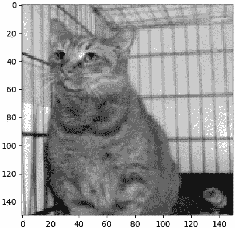
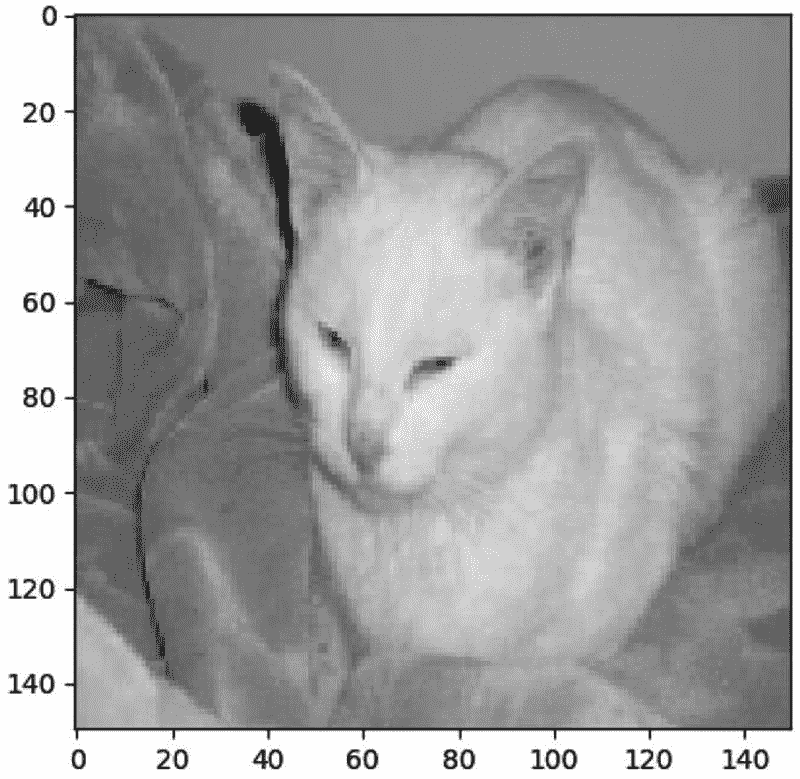
在这个例子中，我们将使用卷积神经网络来构建一个狗和猫的图像分类器。我们将使用一个流行的数据集，它是由 Francois Chollet 推广的，由微软研究院提供，可从 Kaggle 获得。 ^xxxv 和 MNIST 数据集一样，这个数据集在研究中被广泛使用。它包含 12，500 个猫图像和 12，500 个狗图像，尽管我们将只为每个类使用 2000 个图像(总共 4000 个图像)来加速训练。我们将使用 500 张猫图像和 500 张狗图像(总共 1000 张图像)进行测试。见图 7-11 。

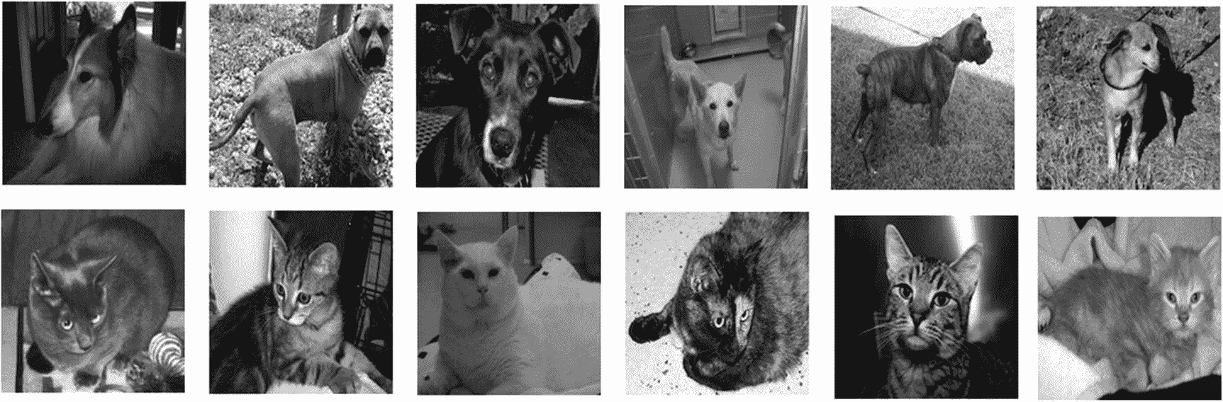
图 7-11

来自数据集的样本狗和猫图像

我们将使用 fit_generator 来训练我们的 Keras 模型。我们还将利用 ImageDataGenerator 类来批量加载数据，从而允许我们处理大量数据。如果您的大型数据集无法容纳在内存中，并且您没有访问分布式环境的权限，这将非常有用。使用 ImageDataGenerator 的另一个好处是，它能够执行随机数据转换来扩充您的数据，帮助模型更好地进行概括，并帮助防止过度拟合。这个例子将展示如何在不使用 Spark 的情况下使用 Keras 的大型数据集。参见清单 7-6 。

import matplotlib.pyplot as plt
import numpy as np
import cv2

from keras.preprocessing.image import ImageDataGenerator
from keras.preprocessing import image
from keras.models import Sequential
from keras.layers import Conv2D, MaxPooling2D
from keras.layers import Activation, Dropout, Flatten, Dense
from keras import backend as K

# The image dimension is 150x150\. RGB = 3.

if K.image_data_format() == 'channels_first':
    input_shape = (3, 150, 150)
else:
    input_shape = (150, 150, 3)

model = Sequential()

model.add(Conv2D(32, (3, 3), input_shape=input_shape, activation="relu"))
model.add(MaxPooling2D(pool_size=(2, 2)))

model.add(Conv2D(32, (3, 3), activation="relu"))
model.add(MaxPooling2D(pool_size=(2, 2)))

model.add(Conv2D(64, (3, 3), activation="relu"))
model.add(MaxPooling2D(pool_size=(2, 2)))

model.add(Flatten())
model.add(Dense(64, activation="relu"))
model.add(Dropout(0.5))
model.add(Dense(1, activation="sigmoid"))

# Compile the model.

model.compile(loss='binary_crossentropy',
              optimizer='rmsprop',
              metrics=['accuracy'])

print(model.summary())

_________________________________________________________________
Layer (type)                 Output Shape              Param #
=================================================================
conv2d_1 (Conv2D)            (None, 148, 148, 32)      896
_________________________________________________________________
max_pooling2d_1 (MaxPooling2 (None, 74, 74, 32)        0
_________________________________________________________________
conv2d_2 (Conv2D)            (None, 72, 72, 32)        9248
_________________________________________________________________
max_pooling2d_2 (MaxPooling2 (None, 36, 36, 32)        0
_________________________________________________________________
conv2d_3 (Conv2D)            (None, 34, 34, 64)        18496
_________________________________________________________________
max_pooling2d_3 (MaxPooling2 (None, 17, 17, 64)        0
_________________________________________________________________
flatten_1 (Flatten)          (None, 18496)             0
_________________________________________________________________
dense_1 (Dense)              (None, 64)                1183808
_________________________________________________________________
dropout_1 (Dropout)          (None, 64)                0
_________________________________________________________________
dense_2 (Dense)              (None, 1)                 65
=================================================================
Total params: 1,212,513
Trainable params: 1,212,513
Non-trainable params: 0
_________________________________________________________________
None

# We will use the following augmentation configuration for training.

train_datagen = ImageDataGenerator(
    rescale=1\. / 255,
    width_shift_range=0.2,
    height_shift_range=0.2,
    horizontal_flip=True)

# The only augmentation for test data is rescaling.

test_datagen = ImageDataGenerator(rescale=1\. / 255)

train_generator = train_datagen.flow_from_directory(
    '/data/train',
    target_size=(150, 150),
    batch_size=16,
    class_mode='binary')

Found 4000 images belonging to 2 classes.

validation_generator = test_datagen.flow_from_directory(
    '/data/test',
    target_size=(150, 150),
    batch_size=16,
    class_mode='binary')

Found 1000 images belonging to 2 classes.

# steps_per_epoch should be set to the total number of training sample,
# while validation_steps is set to the number of test samples. We set
# epoch to 15, steps_per_epoch and validation_steps to 100 to expedite
# model training.

model.fit_generator(
    train_generator,
    steps_per_epoch=100,
    epochs=1=25,
    validation_data=validation_generator,
    validation_steps=100)

Epoch 1/25
100/100 [==============================] - 45s 451ms/step - loss: 0.6439 - acc: 0.6244 - val_loss: 0.5266 - val_acc: 0.7418
Epoch 2/25
100/100 [==============================] - 44s 437ms/step - loss: 0.6259 - acc: 0.6681 - val_loss: 0.5577 - val_acc: 0.7304
Epoch 3/25

100/100 [==============================] - 43s 432ms/step - loss: 0.6326 - acc: 0.6338 - val_loss: 0.5922 - val_acc: 0.7029
Epoch 4/25
100/100 [==============================] - 43s 434ms/step - loss: 0.6538 - acc: 0.6300 - val_loss: 0.5642 - val_acc: 0.7052
Epoch 5/25
100/100 [==============================] - 44s 436ms/step - loss: 0.6263 - acc: 0.6600 - val_loss: 0.6725 - val_acc: 0.6746
Epoch 6/25
100/100 [==============================] - 43s 427ms/step - loss: 0.6229 - acc: 0.6606 - val_loss: 0.5586 - val_acc: 0.7538
Epoch 7/25
100/100 [==============================] - 43s 426ms/step - loss: 0.6470 - acc: 0.6562 - val_loss: 0.5878 - val_acc: 0.7077
Epoch 8/25
100/100 [==============================] - 43s 429ms/step - loss: 0.6524 - acc: 0.6437 - val_loss: 0.6414 - val_acc: 0.6539
Epoch 9/25
100/100 [==============================] - 43s 427ms/step - loss: 0.6131 - acc: 0.6831 - val_loss: 0.5636 - val_acc: 0.7304
Epoch 10/25
100/100 [==============================] - 43s 429ms/step - loss: 0.6293 - acc: 0.6538 - val_loss: 0.5857 - val_acc: 0.7186
Epoch 11/25
100/100 [==============================] - 44s 437ms/step - loss: 0.6207 - acc: 0.6713 - val_loss: 0.5467 - val_acc: 0.7279
Epoch 12/25
100/100 [==============================] - 43s 430ms/step - loss: 0.6131 - acc: 0.6587 - val_loss: 0.5279 - val_acc: 0.7348
Epoch 13/25
100/100 [==============================] - 43s 428ms/step - loss: 0.6090 - acc: 0.6781 - val_loss: 0.6221 - val_acc: 0.7054
Epoch 14/25
100/100 [==============================] - 42s 421ms/step - loss: 0.6273 - acc: 0.6756 - val_loss: 0.5446 - val_acc: 0.7506
Epoch 15/25
100/100 [==============================] - 44s 442ms/step - loss: 0.6139 - acc: 0.6775 - val_loss: 0.6073 - val_acc: 0.6954
Epoch 16/25
100/100 [==============================] - 44s 441ms/step - loss: 0.6080 - acc: 0.6806 - val_loss: 0.5365 - val_acc: 0.7437
Epoch 17/25
100/100 [==============================] - 45s 448ms/step - loss: 0.6225 - acc: 0.6719 - val_loss: 0.5831 - val_acc: 0.6935
Epoch 18/25
100/100 [==============================] - 43s 428ms/step - loss: 0.6124 - acc: 0.6769 - val_loss: 0.5457 - val_acc: 0.7361
Epoch 19/25
100/100 [==============================] - 43s 430ms/step - loss: 0.6061 - acc: 0.6844 - val_loss: 0.5587 - val_acc: 0.7399
Epoch 20/25
100/100 [==============================] - 43s 429ms/step - loss: 0.6209 - acc: 0.6613 - val_loss: 0.5699 - val_acc: 0.7280
Epoch 21/25
100/100 [==============================] - 43s 428ms/step - loss: 0.6252 - acc: 0.6650 - val_loss: 0.5550 - val_acc: 0.7247
Epoch 22/25
100/100 [==============================] - 43s 429ms/step - loss: 0.6306 - acc: 0.6594 - val_loss: 0.5466 - val_acc: 0.7236
Epoch 23/25

100/100 [==============================] - 43s 427ms/step - loss: 0.6086 - acc: 0.6819 - val_loss: 0.5790 - val_acc: 0.6824
Epoch 24/25
100/100 [==============================] - 43s 425ms/step - loss: 0.6059 - acc: 0.7000 - val_loss: 0.5433 - val_acc: 0.7197
Epoch 25/25
100/100 [==============================] - 43s 426ms/step - loss: 0.6261 - acc: 0.6794 - val_loss: 0.5987 - val_acc: 0.7167
<keras.callbacks.History object at 0x7ff72c7c3890>

# We get a 71% validation accuracy. To increase model accuracy, you can try several things such as adding more training data and increasing the number of epochs.

model.save_weights('dogs_vs_cats.h5')

# Let's now use our model to classify a few images. dogs=1, cats=0

# Let's start with dogs.
img = cv2.imread(“/data/test/dogs/dog.148.jpg")

img = np.array(img).astype('float32')/255
img = cv2.resize(img, (150,150))
plt.imshow(img)
plt.show()

Listing 7-6Using ImageDataGenerator and Fit_Generator

img = img.reshape(1, 150, 150, 3)

print(model.predict(img))
[[0.813732]]

print(round(model.predict(img)))
1.0

# Another one
img = cv2.imread("/data/test/dogs/dog.235.jpg")

img = np.array(img).astype('float32')/255
img = cv2.resize(img, (150,150))
plt.imshow(img)
plt.show()

img = img.reshape(1, 150, 150, 3)

print(model.predict(img))
[[0.92639965]]

print(round(model.predict(img)))
1.0

# Let's try some cat photos.

img = cv2.imread("/data/test/cats/cat.355.jpg")

img = np.array(img).astype('float32')/255
img = cv2.resize(img, (150,150))
plt.imshow(img)
plt.show()

img = img.reshape(1, 150, 150, 3)

print(model.predict(img))
[[0.49332634]]

print(round(model.predict(img)))
0.0

# Another one
img = cv2.imread("/data/test/cats/cat.371.jpg")

img = np.array(img).astype('float32')/255
img = cv2.resize(img, (150,150))
plt.imshow(img)
plt.show()

img = img.reshape(1, 150, 150, 3)

print(model.predict(img))
[[0.16990553]]

print(round(model.predict(img)))
0.0

摘要

这一章为你提供了深度学习和 Spark 分布式深度学习的介绍。我选择 Keras 进行深度学习是因为它简单、易用、受欢迎。我选择 Elephas 和 Dist-Keras 进行分布式深度学习，以保持 Keras 的易用性，同时通过 Spark 实现高度可扩展的深度学习工作负载。除了 Elephas 和 Dist-Keras，我建议您探索其他非 Spark 分布式深度学习框架，如 Horovod。对于深度学习的更深入的处理，我推荐弗朗索瓦·乔莱(曼宁)的用 Python 深度学习和伊恩·古德菲勒、约舒阿·本吉奥和亚伦·库维尔(麻省理工出版社)的深度学习。

参考

1. 弗朗西斯·克里克，《惊人的假设:对灵魂的科学探索》，斯克里布纳，1995 年

2. 迈克尔·科普兰；“人工智能、机器学习、深度学习有什么区别？”，nvidia.com，2016， https://blogs.nvidia.com/blog/2016/07/29/whats-difference-artificial-intelligence-machine-learning-deep-learning-ai/

3. 英伟达；《深度学习》，developer.nvidia.com，2019， https://developer.nvidia.com/deep-learning

4. 心灵深处；“Alpha Go，”deepmind.com，2019 年，

5. 特斯拉；《驾驶的未来》，tesla.com，2019， www.tesla.com/autopilot

6. 罗布·孔戈；“特斯拉提高了自动驾驶汽车制造商的门槛，”nvidia.com，2019 年， https://blogs.nvidia.com/blog/2019/04/23/tesla-self-driving/

7. SAS《神经网络如何工作》，sas.com，2019， www.sas.com/en_us/insights/analytics/neural-networks.html

8. H2O；《深度学习(神经网络)》，h2o.ai，2019， http://docs.h2o.ai/h2o/latest-stable/h2o-docs/data-science/deep-learning.html

9. 迈克尔·马尔萨利；《麦卡洛克-皮茨神经元》，ilstu.edu，2019， www.mind.ilstu.edu/curriculum/modOverview.php?modGUI=212

10. 弗朗西斯·克里克；《大脑损伤》第 181 页，西蒙&舒斯特，1995 年,《惊人的假设:对灵魂的科学探索》

11. 大卫·b·福格尔；定义人工智能第 20 页，Wiley，2005,《进化计算:走向机器智能的新哲学》,第三版

12. 巴纳巴斯·波佐斯；《机器学习导论(讲义)感知器》，cmu.edu，2017， www.cs.cmu.edu/~10701/slides/Perceptron_Reading_Material.pdf

13. SAS《神经网络的历史》，sas.com，2019， www.sas.com/en_us/insights/analytics/neural-networks.html

14. Skymind《神经网络反向传播初学者指南》，skymind.ai，2019， https://skymind.ai/wiki/backpropagation

15. Cognilytica“人们是否过度迷恋深度学习，它真的能实现吗？”，cognilytica.com，2018， www.cognilytica.com/2018/07/10/are-people-overly-infatuated-with-deep-learning-and-can-it-really-deliver/

16. Yann LeCun“不变量识别:卷积神经网络”，lecun.com，2004， http://yann.lecun.com/ex/research/index.html

17. 凯尔·威格斯；“Geoffrey Hinton、Yann LeCun、Yoshua Bengio 获图灵奖”，venturebeat.com，2019， https://venturebeat.com/2019/03/27/geoffrey-hinton-yann-lecun-and-yoshua-bengio-honored-with-the-turing-award/

18. 亚历克斯·克里热夫斯基、伊利亚·苏茨基弗、杰弗里·欣顿；“用深度卷积神经网络进行 ImageNet 分类”，toronto.edu，2012， www.cs.toronto.edu/~fritz/absps/imagenet.pdf

19. 皮托奇；“Alexnet，”pytorch.org，2019 年，

20. 弗朗索瓦·乔莱；“计算机视觉的深度学习”，2018，用 Python 进行深度学习

21. 安德烈·卡帕西；《卷积神经网络(CNN/conv nets)》，github.io，2019， http://cs231n.github.io/convolutional-networks/

22. 杰尼尔·达拉勒和索希尔·帕特尔；“图像基础”，Packt 出版社，2013 年，即时 OpenCV Starter

23. MATLAB《用 MATLAB 介绍深度学习》。mathworks.com，2019， www.mathworks.com/content/dam/mathworks/tag-team/Objects/d/80879v00_Deep_Learning_ebook.pdf

24. 文森特·杜穆林和弗朗切斯科·维辛；《深度卷积运算指南》

学，《axiv.org》2018， [`https://arxiv.org/pdf/1603.07285.pdf`](https://arxiv.org/pdf/1603.07285.pdf)

25. 阿尼什·辛格·瓦利亚；“激活函数及其类型——哪个更好？”，towardsdatascience.com，2017， https://towardsdatascience.com/activation-functions-and-its-types-which-is-better-a9a5310cc8f

26. Skymind《AI 框架比较》，skymind.ai，2019， https://skymind.ai/wiki/comparison-frameworks-dl4j-tensorflow-pytorch

27. 尼哈尔·加贾雷；“Keras + TensorFlow 中的简单神经网络对虹膜数据集进行分类”，github.com，2017， https://gist.github.com/NiharG15/cd8272c9639941cf8f481a7c4478d525

28. 大 dl；“什么是重头戏，”github.com，2019 年，

29. Skymind《分布式深度学习，第一部分:神经网络分布式训练导论》，skymind.ai，2017， https://blog.skymind.ai/distributed-deep-learning-part-1-an-introduction-to-distributed-training-of-neural-networks/

30. Skymind《分布式深度学习，第一部分:神经网络分布式训练导论》，skymind.ai，2017， https://blog.skymind.ai/distributed-deep-learning-part-1-an-introduction-to-distributed-training-of-neural-networks/

31. 数据块；“Apache Spark 的深度学习管道”，github.com，2019， https://github.com/databricks/spark-deep-learning

32. Max Pumperla“Elephas:分布式深度学习与 Keras & Spark”，github.com，2019， https://github.com/maxpumperla/elephas

33. max pumbaa 她；" mnist_lp_spark.py，" github.com，2019 年，

34. 游里·r·赫尔曼斯，欧洲粒子物理研究所信息技术数据库；《分布式 Keras:使用 Apache Spark 和 Keras 的分布式深度学习》，Github.com，2016， https://github.com/JoeriHermans/dist-keras/

35. 微软研究院；《狗与猫》，Kaggle.com，2013， www.kaggle.com/c/dogs-vs-cats/data

36. 弗朗索瓦·乔莱；“用极少的数据构建强大的图像分类模型”，keras.io，2016， https://blog.keras.io/building-powerful-image-classification-models-using-very-little-data.html