


使用 Python 和 Keras 逐步开发第一个神经网络
原文:
machinelearningmastery.com/tutorial-first-neural-network-python-keras/
Keras 是一个功能强大且易于使用的 Python 库,用于开发和评估深度学习模型。
它包含了高效的数值计算库 Theano 和 TensorFlow,允许您在几行代码中定义和训练神经网络模型。
在这篇文章中,您将了解如何使用 Keras 在 Python 中创建第一个神经网络模型。
让我们开始吧。
- 2017 年 2 月更新:更新了预测示例,因此在 Python 2 和 Python 3 中可以进行舍入。
- 2017 年 3 月更新:更新了 Keras 2.0.2,TensorFlow 1.0.1 和 Theano 0.9.0 的示例。
- 更新 Mar / 2018 :添加了备用链接以下载数据集,因为原始图像已被删除。

使用 Keras 逐步开发 Python 中的第一个神经网络
Phil Whitehouse 的照片,保留一些权利。
教程概述
不需要很多代码,但我们会慢慢跨过它,以便您知道将来如何创建自己的模型。
您将在本教程中介绍的步骤如下:
- 加载数据。
- 定义模型。
- 编译模型。
- 适合模型。
- 评估模型。
- 把它绑在一起。
本教程有一些要求:
- 您已安装并配置了 Python 2 或 3。
- 您已安装并配置了 SciPy(包括 NumPy)。
- 您安装并配置了 Keras 和后端(Theano 或 TensorFlow)。
如果您需要有关环境的帮助,请参阅教程:
创建一个名为 keras_first_network.py 的新文件,然后在您输入时将代码输入或复制并粘贴到文件中。
1.加载数据
每当我们使用使用随机过程(例如随机数)的机器学习算法时,最好设置随机数种子。
这样您就可以反复运行相同的代码并获得相同的结果。如果您需要演示结果,使用相同的随机源比较算法或调试代码的一部分,这非常有用。
您可以使用您喜欢的任何种子初始化随机数生成器,例如:
from keras.models import Sequential
from keras.layers import Dense
import numpy
# fix random seed for reproducibility
numpy.random.seed(7)
现在我们可以加载我们的数据。
在本教程中,我们将使用 Pima Indians 糖尿病数据集。这是来自 UCI 机器学习库的标准机器学习数据集。它描述了皮马印第安人的患者病历数据,以及他们是否在五年内患有糖尿病。
因此,它是二分类问题(糖尿病发作为 1 或不为 0)。描述每个患者的所有输入变量都是数字的。这使得它可以直接用于期望数字输入和输出值的神经网络,是我们在 Keras 的第一个神经网络的理想选择。
下载数据集并将其放在本地工作目录中,与 python 文件相同。使用文件名保存:
pima-indians-diabetes.csv
您现在可以使用 NumPy 函数 **loadtxt()**直接加载文件。有八个输入变量和一个输出变量(最后一列)。加载后,我们可以将数据集拆分为输入变量(X)和输出类变量(Y)。
# load pima indians dataset
dataset = numpy.loadtxt("pima-indians-diabetes.csv", delimiter=",")
# split into input (X) and output (Y) variables
X = dataset[:,0:8]
Y = dataset[:,8]
我们初始化了随机数生成器,以确保我们的结果可重现并加载我们的数据。我们现在准备定义我们的神经网络模型。
请注意,数据集有 9 列,范围 0:8 将选择 0 到 7 之间的列,在索引 8 之前停止。如果这对您来说是新的,那么您可以在此帖子中了解有关数组切片和范围的更多信息:
2.定义模型
Keras 中的模型被定义为层序列。
我们创建一个 Sequential 模型并一次添加一个层,直到我们对网络拓扑感到满意为止。
要做的第一件事是确保输入层具有正确数量的输入。当使用 input_dim 参数创建第一层并为 8 个输入变量将其设置为 8 时,可以指定此项。
我们如何知道层数及其类型?
这是一个非常难的问题。我们可以使用启发式方法,通常通过试验和错误实验的过程找到最好的网络结构。通常,如果有任何帮助,您需要一个足够大的网络来捕获问题的结构。
在此示例中,我们将使用具有三个层的完全连接的网络结构。
完全连接的层使用 Dense 类定义。我们可以指定层中神经元的数量作为第一个参数,初始化方法作为 init 指定第二个参数,并使用激活参数指定激活函数。
在这种情况下,我们将网络权重初始化为从均匀分布(’ uniform ')生成的小随机数,在这种情况下介于 0 和 0.05 之间,因为这是 Keras 中的默认均匀权重初始化。对于从高斯分布产生的小随机数,另一种传统的替代方案是’正常’。
我们将在前两层使用整流器(’ relu ')激活函数,在输出层使用 sigmoid 函数。过去,所有层都优先选择 sigmoid 和 tanh 激活函数。目前,使用整流器激活功能可以获得更好的表现。我们在输出层使用 sigmoid 来确保我们的网络输出介于 0 和 1 之间,并且很容易映射到 1 级概率或者使用默认阈值 0.5 捕捉到任一类的硬分类。
我们可以通过添加每一层将它们拼凑在一起。第一层有 12 个神经元,需要 8 个输入变量。第二个隐藏层有 8 个神经元,最后,输出层有 1 个神经元来预测类别(是否发生糖尿病)。
# create model
model = Sequential()
model.add(Dense(12, input_dim=8, activation='relu'))
model.add(Dense(8, activation='relu'))
model.add(Dense(1, activation='sigmoid'))
3.编译模型
既然定义了模型,我们就可以编译它。
编译模型使用封面下的高效数字库(所谓的后端),如 Theano 或 TensorFlow。后端自动选择最佳方式来表示网络以进行训练并使预测在硬件上运行,例如 CPU 或 GPU 甚至分布式。
编译时,我们必须指定训练网络时所需的一些其他属性。记住训练网络意味着找到最佳权重集来预测这个问题。
我们必须指定用于评估一组权重的损失函数,用于搜索网络的不同权重的优化器以及我们希望在训练期间收集和报告的任何可选指标。
在这种情况下,我们将使用对数损失,对于二分类问题,在 Keras 中定义为“ binary_crossentropy ”。我们还将使用有效的梯度下降算法“ adam ”,因为它是一个有效的默认值。在“ Adam:随机优化方法”一文中了解有关 Adam 优化算法的更多信息。
最后,因为它是一个分类问题,我们将收集并报告分类准确度作为指标。
# Compile model
model.compile(loss='binary_crossentropy', optimizer='adam', metrics=['accuracy'])
4.适合模型
我们已经定义了我们的模型并将其编译为高效计算。
现在是时候在一些数据上执行模型了。
我们可以通过调用模型上的 **fit()**函数来训练或拟合我们的加载数据模型。
训练过程将通过名为 epochs 的数据集进行固定次数的迭代,我们必须使用 nepochs 参数指定。我们还可以设置在执行网络中的权重更新之前评估的实例数,称为批量大小并使用 batch_size 参数进行设置。
对于这个问题,我们将运行少量迭代(150)并使用相对较小的批量大小 10.再次,这些可以通过试验和错误通过实验选择。
# Fit the model
model.fit(X, Y, epochs=150, batch_size=10)
这是工作在 CPU 或 GPU 上发生的地方。
此示例不需要 GPU,但如果您对如何在云中廉价地在 GPU 硬件上运行大型模型感兴趣,请参阅此帖子:
5.评估模型
我们已经在整个数据集上训练了神经网络,我们可以在同一数据集上评估网络的表现。
这只会让我们了解我们对数据集建模的程度(例如训练精度),但不知道算法在新数据上的表现如何。我们这样做是为了简化,但理想情况下,您可以将数据分成训练和测试数据集,以便对模型进行训练和评估。
您可以使用模型上的 **evaluate()**函数在训练数据集上评估模型,并将其传递给用于训练模型的相同输入和输出。
这将为每个输入和输出对生成预测并收集分数,包括平均损失和您配置的任何指标,例如准确率。
# evaluate the model
scores = model.evaluate(X, Y)
print("\n%s: %.2f%%" % (model.metrics_names[1], scores[1]*100))
6.将它们结合在一起
您刚刚看到了如何在 Keras 中轻松创建第一个神经网络模型。
让我们将它们组合成一个完整的代码示例。
# Create your first MLP in Keras
from keras.models import Sequential
from keras.layers import Dense
import numpy
# fix random seed for reproducibility
numpy.random.seed(7)
# load pima indians dataset
dataset = numpy.loadtxt("pima-indians-diabetes.csv", delimiter=",")
# split into input (X) and output (Y) variables
X = dataset[:,0:8]
Y = dataset[:,8]
# create model
model = Sequential()
model.add(Dense(12, input_dim=8, activation='relu'))
model.add(Dense(8, activation='relu'))
model.add(Dense(1, activation='sigmoid'))
# Compile model
model.compile(loss='binary_crossentropy', optimizer='adam', metrics=['accuracy'])
# Fit the model
model.fit(X, Y, epochs=150, batch_size=10)
# evaluate the model
scores = model.evaluate(X, Y)
print("\n%s: %.2f%%" % (model.metrics_names[1], scores[1]*100))
运行此示例,您应该看到 150 个迭代中的每个迭代记录每个历史记录的丢失和准确率的消息,然后对训练数据集上的训练模型进行最终评估。
在带有 Theano 后端的 CPU 上运行的工作站上执行大约需要 10 秒钟。
...
Epoch 145/150
768/768 [==============================] - 0s - loss: 0.5105 - acc: 0.7396
Epoch 146/150
768/768 [==============================] - 0s - loss: 0.4900 - acc: 0.7591
Epoch 147/150
768/768 [==============================] - 0s - loss: 0.4939 - acc: 0.7565
Epoch 148/150
768/768 [==============================] - 0s - loss: 0.4766 - acc: 0.7773
Epoch 149/150
768/768 [==============================] - 0s - loss: 0.4883 - acc: 0.7591
Epoch 150/150
768/768 [==============================] - 0s - loss: 0.4827 - acc: 0.7656
 32/768 [>.............................] - ETA: 0s
acc: 78.26%
注意:如果您尝试在 IPython 或 Jupyter 笔记本中运行此示例,则可能会出错。原因是训练期间的输出进度条。您可以通过在 **model.fit()**的调用中设置 verbose = 0 来轻松关闭它们。
请注意,您的模型的技能可能会有所不同。
神经网络是一种随机算法,意味着相同数据上的相同算法可以训练具有不同技能的不同模型。这是一个功能,而不是一个 bug。您可以在帖子中了解更多相关信息:
我们确实尝试修复随机种子以确保您和我获得相同的模型,因此得到相同的结果,但这并不总是适用于所有系统。我在这里写了更多关于使用 Keras 模型再现结果的问题。
7.奖金:做出预测
我被问到的头号问题是:
在训练我的模型后,如何使用它来预测新数据?
好问题。
我们可以调整上面的示例并使用它来生成训练数据集的预测,假装它是我们以前从未见过的新数据集。
做出预测就像调用 **model.predict()**一样简单。我们在输出层使用 sigmoid 激活函数,因此预测将在 0 到 1 之间的范围内。我们可以通过舍入它们轻松地将它们转换为这个分类任务的清晰二元预测。
下面列出了为训练数据中的每条记录做出预测的完整示例。
# Create first network with Keras
from keras.models import Sequential
from keras.layers import Dense
import numpy
# fix random seed for reproducibility
seed = 7
numpy.random.seed(seed)
# load pima indians dataset
dataset = numpy.loadtxt("pima-indians-diabetes.csv", delimiter=",")
# split into input (X) and output (Y) variables
X = dataset[:,0:8]
Y = dataset[:,8]
# create model
model = Sequential()
model.add(Dense(12, input_dim=8, init='uniform', activation='relu'))
model.add(Dense(8, init='uniform', activation='relu'))
model.add(Dense(1, init='uniform', activation='sigmoid'))
# Compile model
model.compile(loss='binary_crossentropy', optimizer='adam', metrics=['accuracy'])
# Fit the model
model.fit(X, Y, epochs=150, batch_size=10,  verbose=2)
# calculate predictions
predictions = model.predict(X)
# round predictions
rounded = [round(x[0]) for x in predictions]
print(rounded)
现在运行此修改示例将打印每个输入模式的预测。如果需要,我们可以直接在我们的应用程序中使用这些预测
[1.0, 0.0, 1.0, 0.0, 1.0, 0.0, 0.0, 1.0, 1.0, 0.0, 0.0, 1.0, 1.0, 1.0, 1.0, 0.0, 1.0, 0.0, 0.0, 0.0, 1.0, 0.0, 1.0, 0.0, 1.0, 1.0, 1.0, 0.0, 0.0, 0.0, 0.0, 1.0, 0.0, 0.0, 1.0, 0.0, 1.0, 1.0, 0.0, 1.0, 1.0, 1.0, 0.0, 1.0, 1.0, 1.0, 1.0, 0.0, 1.0, 0.0, 0.0, 0.0, 0.0, 1.0, 1.0, 0.0, 1.0, 0.0, 1.0, 0.0, 0.0, 1.0, 0.0, 1.0, 1.0, 0.0, 0.0, 1.0, 0.0, 0.0, 0.0, 1.0, 1.0, 0.0, 0.0, 0.0, 0.0, 0.0, 1.0, 0.0, 0.0, 0.0, 0.0, 0.0, 0.0, 0.0, 1.0, 0.0, 1.0, 0.0, 0.0, 0.0, 0.0, 0.0, 0.0, 1.0, 0.0, 0.0, 0.0, 1.0, 1.0, 0.0, 0.0, 0.0, 0.0, 0.0, 0.0, 1.0, 0.0, 0.0, 1.0, 1.0, 0.0, 0.0, 1.0, 1.0, 1.0, 0.0, 0.0, 0.0, 1.0, 0.0, 0.0, 0.0, 0.0, 0.0, 0.0, 0.0, 0.0, 0.0, 1.0, 1.0, 1.0, 0.0, 0.0, 0.0, 0.0, 0.0, 0.0, 0.0, 0.0, 0.0, 0.0, 1.0, 1.0, 0.0, 0.0, 0.0, 1.0, 0.0, 1.0, 0.0, 1.0, 1.0, 1.0, 1.0, 0.0, 0.0, 0.0, 1.0, 0.0, 0.0, 0.0, 0.0, 0.0, 0.0, 1.0, 1.0, 0.0, 0.0, 0.0, 1.0, 0.0, 0.0, 0.0, 1.0, 0.0, 0.0, 1.0, 1.0, 0.0, 0.0, 0.0, 0.0, 1.0, 1.0, 1.0, 0.0, 0.0, 1.0, 0.0, 1.0, 1.0, 1.0, 0.0, 1.0, 0.0, 0.0, 0.0, 1.0, 0.0, 0.0, 0.0, 0.0, 0.0, 0.0, 1.0, 1.0, 0.0, 1.0, 0.0, 0.0, 1.0, 0.0, 1.0, 1.0, 0.0, 1.0, 0.0, 1.0, 0.0, 1.0, 0.0, 0.0, 0.0, 0.0, 0.0, 1.0, 1.0, 0.0, 1.0, 1.0, 0.0, 1.0, 0.0, 1.0, 1.0, 1.0, 1.0, 0.0, 0.0, 0.0, 1.0, 1.0, 1.0, 1.0, 1.0, 0.0, 1.0, 0.0, 0.0, 0.0, 0.0, 0.0, 1.0, 0.0, 0.0, 0.0, 1.0, 1.0, 1.0, 1.0, 0.0, 1.0, 1.0, 0.0, 1.0, 1.0, 0.0, 1.0, 1.0, 0.0, 0.0, 0.0, 0.0, 0.0, 0.0, 0.0, 0.0, 0.0, 1.0, 1.0, 0.0, 1.0, 0.0, 1.0, 1.0, 0.0, 0.0, 0.0, 0.0, 0.0, 1.0, 1.0, 0.0, 1.0, 1.0, 0.0, 1.0, 0.0, 1.0, 1.0, 0.0, 0.0, 0.0, 0.0, 1.0, 0.0, 0.0, 0.0, 0.0, 0.0, 0.0, 0.0, 1.0, 0.0, 0.0, 1.0, 0.0, 1.0, 0.0, 0.0, 0.0, 1.0, 0.0, 0.0, 0.0, 1.0, 0.0, 0.0, 1.0, 0.0, 1.0, 0.0, 0.0, 1.0, 0.0, 1.0, 1.0, 1.0, 0.0, 0.0, 0.0, 0.0, 0.0, 0.0, 0.0, 1.0, 0.0, 0.0, 0.0, 0.0, 0.0, 0.0, 0.0, 1.0, 1.0, 1.0, 0.0, 1.0, 1.0, 1.0, 0.0, 1.0, 0.0, 0.0, 0.0, 0.0, 0.0, 0.0, 1.0, 0.0, 0.0, 0.0, 1.0, 1.0, 0.0, 0.0, 1.0, 0.0, 0.0, 0.0, 0.0, 0.0, 0.0, 0.0, 0.0, 0.0, 1.0, 0.0, 0.0, 1.0, 0.0, 0.0, 1.0, 0.0, 0.0, 0.0, 0.0, 1.0, 0.0, 0.0, 0.0, 0.0, 1.0, 1.0, 0.0, 0.0, 1.0, 1.0, 0.0, 0.0, 0.0, 0.0, 1.0, 0.0, 0.0, 1.0, 0.0, 0.0, 0.0, 0.0, 0.0, 0.0, 1.0, 1.0, 0.0, 1.0, 0.0, 0.0, 0.0, 0.0, 0.0, 0.0, 0.0, 1.0, 1.0, 1.0, 0.0, 0.0, 1.0, 0.0, 0.0, 1.0, 1.0, 1.0, 0.0, 0.0, 0.0, 0.0, 0.0, 0.0, 0.0, 0.0, 0.0, 1.0, 0.0, 0.0, 1.0, 0.0, 0.0, 0.0, 0.0, 0.0, 0.0, 0.0, 0.0, 0.0, 0.0, 1.0, 1.0, 0.0, 0.0, 1.0, 0.0, 0.0, 0.0, 0.0, 0.0, 0.0, 1.0, 0.0, 0.0, 0.0, 1.0, 1.0, 1.0, 1.0, 0.0, 1.0, 0.0, 0.0, 0.0, 1.0, 0.0, 0.0, 0.0, 0.0, 1.0, 1.0, 0.0, 0.0, 0.0, 0.0, 0.0, 0.0, 1.0, 0.0, 0.0, 0.0, 0.0, 0.0, 0.0, 0.0, 0.0, 1.0, 1.0, 1.0, 0.0, 0.0, 0.0, 0.0, 0.0, 1.0, 1.0, 0.0, 0.0, 0.0, 0.0, 0.0, 0.0, 0.0, 0.0, 0.0, 0.0, 1.0, 0.0, 0.0, 0.0, 1.0, 1.0, 0.0, 0.0, 0.0, 0.0, 1.0, 1.0, 0.0, 0.0, 1.0, 0.0, 0.0, 0.0, 0.0, 0.0, 1.0, 0.0, 0.0, 1.0, 0.0, 1.0, 1.0, 0.0, 0.0, 0.0, 0.0, 0.0, 0.0, 1.0, 0.0, 0.0, 0.0, 0.0, 0.0, 0.0, 0.0, 1.0, 0.0, 1.0, 1.0, 0.0, 0.0, 0.0, 1.0, 1.0, 0.0, 1.0, 0.0, 1.0, 0.0, 1.0, 0.0, 1.0, 0.0, 1.0, 0.0, 0.0, 0.0, 1.0, 0.0, 0.0, 0.0, 0.0, 1.0, 1.0, 1.0, 1.0, 0.0, 0.0, 0.0, 0.0, 1.0, 1.0, 0.0, 1.0, 0.0, 0.0, 0.0, 1.0, 1.0, 0.0, 0.0, 1.0, 0.0, 0.0, 0.0, 0.0, 0.0, 1.0, 0.0, 1.0, 0.0, 0.0, 0.0, 0.0, 1.0, 0.0, 0.0, 0.0, 0.0, 0.0, 0.0, 1.0, 0.0, 0.0, 1.0, 1.0, 1.0, 1.0, 0.0, 0.0, 0.0, 0.0, 1.0, 0.0, 1.0, 0.0, 1.0, 1.0, 0.0, 1.0, 1.0, 1.0, 1.0, 1.0, 0.0, 0.0, 1.0, 1.0, 1.0, 1.0, 0.0, 0.0, 0.0, 0.0, 1.0, 1.0, 0.0, 1.0, 0.0, 0.0, 1.0, 0.0, 0.0, 0.0, 0.0, 0.0, 0.0, 0.0, 1.0, 0.0, 1.0, 0.0, 1.0, 0.0, 1.0, 1.0, 1.0, 0.0, 1.0, 0.0, 1.0, 1.0, 0.0, 0.0, 0.0, 0.0, 0.0, 1.0, 0.0, 0.0, 0.0, 1.0, 0.0, 0.0, 1.0, 1.0, 0.0, 0.0, 0.0, 0.0, 0.0, 1.0, 0.0, 0.0, 0.0, 0.0, 0.0, 0.0, 0.0, 0.0, 0.0, 1.0, 0.0, 0.0, 0.0, 0.0, 0.0, 0.0, 0.0, 1.0, 0.0, 0.0, 1.0, 1.0, 0.0, 1.0, 0.0, 1.0, 1.0, 1.0, 0.0, 0.0, 1.0, 1.0, 0.0, 0.0, 1.0, 0.0, 1.0, 0.0, 1.0, 0.0, 0.0, 0.0, 0.0, 1.0, 0.0]
如果您对使用经过训练的模型做出预测有更多疑问,请参阅此帖子:
摘要
在这篇文章中,您发现了如何使用功能强大的 Keras Python 库创建第一个神经网络模型以进行深度学习。
具体来说,您学习了使用 Keras 创建神经网络或深度学习模型的五个关键步骤,包括:
- 如何加载数据。
- 如何在 Keras 中定义神经网络。
- 如何使用高效的数字后端编译 Keras 模型。
- 如何训练数据模型。
- 如何评估数据模型。
您对 Keras 或本教程有任何疑问吗?
在评论中提出您的问题,我会尽力回答。
相关教程
您是否正在寻找使用 Python 和 Keras 的更多深度学习教程?
看看其中一些:
- Keras 神经网络模型的 5 步生命周期
- 如何使用 Keras 网格搜索 Python 中的深度学习模型的超参数
- Keras 中深度学习的时间序列预测
- Keras 深度学习库的多分类教程
- 使用 Python 中的 Keras 深度学习库进行回归教程
使用 Python 和 Keras 理解有状态 LSTM 循环神经网络
原文:
machinelearningmastery.com/understanding-stateful-lstm-recurrent-neural-networks-python-keras/
强大且流行的递归神经网络是长期短期模型网络或 LSTM。
它被广泛使用,因为该架构克服了困扰所有递归神经网络的消失和暴露梯度问题,允许创建非常大且非常深的网络。
与其他递归神经网络一样,LSTM 网络维持状态,并且在 Keras 框架中如何实现这一点的具体细节可能会令人困惑。
在这篇文章中,您将通过 Keras 深度学习库确切了解 LSTM 网络中的状态。
阅读这篇文章后你会知道:
- 如何为序列预测问题开发一个朴素的 LSTM 网络。
- 如何通过 LSTM 网络批量管理状态和功能。
- 如何在 LSTM 网络中手动管理状态以进行状态预测。
让我们开始吧。
- 2017 年 3 月更新:更新了 Keras 2.0.2,TensorFlow 1.0.1 和 Theano 0.9.0 的示例。
- 更新 Aug / 2018 :更新了 Python 3 的示例,更新了有状态示例以获得 100%的准确率。
- 更新 Mar / 2019 :修正了有状态示例中的拼写错误。

使用 Keras 了解 Python 中的有状态 LSTM 回归神经网络
Martin Abegglen 的照片,保留一些权利。
问题描述:学习字母表
在本教程中,我们将开发和对比许多不同的 LSTM 递归神经网络模型。
这些比较的背景将是学习字母表的简单序列预测问题。也就是说,给定一个字母表的字母,预测字母表的下一个字母。
这是一个简单的序列预测问题,一旦理解就可以推广到其他序列预测问题,如时间序列预测和序列分类。
让我们用一些 python 代码来准备问题,我们可以从示例到示例重用这些代码。
首先,让我们导入我们计划在本教程中使用的所有类和函数。
import numpy
from keras.models import Sequential
from keras.layers import Dense
from keras.layers import LSTM
from keras.utils import np_utils
接下来,我们可以为随机数生成器播种,以确保每次执行代码时结果都相同。
# fix random seed for reproducibility
numpy.random.seed(7)
我们现在可以定义我们的数据集,即字母表。为了便于阅读,我们用大写字母定义字母表。
神经网络模型编号,因此我们需要将字母表的字母映射为整数值。我们可以通过创建字符索引的字典(map)来轻松完成此操作。我们还可以创建反向查找,以便将预测转换回字符以便以后使用。
# define the raw dataset
alphabet = "ABCDEFGHIJKLMNOPQRSTUVWXYZ"
# create mapping of characters to integers (0-25) and the reverse
char_to_int = dict((c, i) for i, c in enumerate(alphabet))
int_to_char = dict((i, c) for i, c in enumerate(alphabet))
现在我们需要创建输入和输出对来训练我们的神经网络。我们可以通过定义输入序列长度,然后从输入字母序列中读取序列来完成此操作。
例如,我们使用输入长度 1.从原始输入数据的开头开始,我们可以读出第一个字母“A”和下一个字母作为预测“B”。我们沿着一个角色移动并重复直到我们达到“Z”的预测。
# prepare the dataset of input to output pairs encoded as integers
seq_length = 1
dataX = []
dataY = []
for i in range(0, len(alphabet) - seq_length, 1):
	seq_in = alphabet[i:i + seq_length]
	seq_out = alphabet[i + seq_length]
	dataX.append([char_to_int[char] for char in seq_in])
	dataY.append(char_to_int[seq_out])
	print(seq_in, '->', seq_out)
我们还打印出输入对以进行健全性检查。
将代码运行到此点将产生以下输出,总结长度为 1 的输入序列和单个输出字符。
A -> B
B -> C
C -> D
D -> E
E -> F
F -> G
G -> H
H -> I
I -> J
J -> K
K -> L
L -> M
M -> N
N -> O
O -> P
P -> Q
Q -> R
R -> S
S -> T
T -> U
U -> V
V -> W
W -> X
X -> Y
Y -> Z
我们需要将 NumPy 数组重新整形为 LSTM 网络所期望的格式,即[_ 样本,时间步长,特征 _]。
# reshape X to be [samples, time steps, features]
X = numpy.reshape(dataX, (len(dataX), seq_length, 1))
一旦重新整形,我们就可以将输入整数归一化到 0 到 1 的范围,即 LSTM 网络使用的 S 形激活函数的范围。
# normalize
X = X / float(len(alphabet))
最后,我们可以将此问题视为序列分类任务,其中 26 个字母中的每一个代表不同的类。因此,我们可以使用 Keras 内置函数 **to_categorical()**将输出(y)转换为单热编码。
# one hot encode the output variable
y = np_utils.to_categorical(dataY)
我们现在准备适应不同的 LSTM 模型。
用于学习 One-Char 到 One-Char 映射的 Naive LSTM
让我们从设计一个简单的 LSTM 开始,学习如何在给定一个字符的上下文的情况下预测字母表中的下一个字符。
我们将问题框架化为单字母输入到单字母输出对的随机集合。正如我们将看到的那样,这是 LSTM 学习问题的难点框架。
让我们定义一个具有 32 个单元的 LSTM 网络和一个具有 softmax 激活功能的输出层,用于做出预测。因为这是一个多分类问题,我们可以使用日志丢失函数(在 Keras 中称为“ categorical_crossentropy ”),并使用 ADAM 优化函数优化网络。
该模型适用于 500 个时期,批量大小为 1。
# create and fit the model
model = Sequential()
model.add(LSTM(32, input_shape=(X.shape[1], X.shape[2])))
model.add(Dense(y.shape[1], activation='softmax'))
model.compile(loss='categorical_crossentropy', optimizer='adam', metrics=['accuracy'])
model.fit(X, y, epochs=500, batch_size=1, verbose=2)
在我们拟合模型之后,我们可以评估和总结整个训练数据集的表现。
# summarize performance of the model
scores = model.evaluate(X, y, verbose=0)
print("Model Accuracy: %.2f%%" % (scores[1]*100))
然后,我们可以通过网络重新运行训练数据并生成预测,将输入和输出对转换回原始字符格式,以便直观地了解网络如何了解问题。
# demonstrate some model predictions
for pattern in dataX:
	x = numpy.reshape(pattern, (1, len(pattern), 1))
	x = x / float(len(alphabet))
	prediction = model.predict(x, verbose=0)
	index = numpy.argmax(prediction)
	result = int_to_char[index]
	seq_in = [int_to_char[value] for value in pattern]
	print(seq_in, "->", result)
下面提供了整个代码清单,以确保完整性。
# Naive LSTM to learn one-char to one-char mapping
import numpy
from keras.models import Sequential
from keras.layers import Dense
from keras.layers import LSTM
from keras.utils import np_utils
# fix random seed for reproducibility
numpy.random.seed(7)
# define the raw dataset
alphabet = "ABCDEFGHIJKLMNOPQRSTUVWXYZ"
# create mapping of characters to integers (0-25) and the reverse
char_to_int = dict((c, i) for i, c in enumerate(alphabet))
int_to_char = dict((i, c) for i, c in enumerate(alphabet))
# prepare the dataset of input to output pairs encoded as integers
seq_length = 1
dataX = []
dataY = []
for i in range(0, len(alphabet) - seq_length, 1):
	seq_in = alphabet[i:i + seq_length]
	seq_out = alphabet[i + seq_length]
	dataX.append([char_to_int[char] for char in seq_in])
	dataY.append(char_to_int[seq_out])
	print(seq_in, '->', seq_out)
# reshape X to be [samples, time steps, features]
X = numpy.reshape(dataX, (len(dataX), seq_length, 1))
# normalize
X = X / float(len(alphabet))
# one hot encode the output variable
y = np_utils.to_categorical(dataY)
# create and fit the model
model = Sequential()
model.add(LSTM(32, input_shape=(X.shape[1], X.shape[2])))
model.add(Dense(y.shape[1], activation='softmax'))
model.compile(loss='categorical_crossentropy', optimizer='adam', metrics=['accuracy'])
model.fit(X, y, epochs=500, batch_size=1, verbose=2)
# summarize performance of the model
scores = model.evaluate(X, y, verbose=0)
print("Model Accuracy: %.2f%%" % (scores[1]*100))
# demonstrate some model predictions
for pattern in dataX:
	x = numpy.reshape(pattern, (1, len(pattern), 1))
	x = x / float(len(alphabet))
	prediction = model.predict(x, verbose=0)
	index = numpy.argmax(prediction)
	result = int_to_char[index]
	seq_in = [int_to_char[value] for value in pattern]
	print(seq_in, "->", result)
运行此示例将生成以下输出。
Model Accuracy: 84.00%
['A'] -> B
['B'] -> C
['C'] -> D
['D'] -> E
['E'] -> F
['F'] -> G
['G'] -> H
['H'] -> I
['I'] -> J
['J'] -> K
['K'] -> L
['L'] -> M
['M'] -> N
['N'] -> O
['O'] -> P
['P'] -> Q
['Q'] -> R
['R'] -> S
['S'] -> T
['T'] -> U
['U'] -> W
['V'] -> Y
['W'] -> Z
['X'] -> Z
['Y'] -> Z
我们可以看到这个问题对于网络来说确实很难学习。
原因是,糟糕的 LSTM 单位没有任何上下文可以使用。每个输入 - 输出模式以随机顺序显示给网络,并且在每个模式(每个批次包含一个模式的每个批次)之后重置网络状态。
这是滥用 LSTM 网络架构,将其视为标准的多层 Perceptron。
接下来,让我们尝试不同的问题框架,以便为网络提供更多的顺序来学习。
Naive LSTM 用于三字符特征窗口到单字符映射
为多层 Perceptrons 添加更多上下文数据的流行方法是使用 window 方法。
这是序列中的先前步骤作为网络的附加输入功能提供的地方。我们可以尝试相同的技巧,为 LSTM 网络提供更多上下文。
在这里,我们将序列长度从 1 增加到 3,例如:
# prepare the dataset of input to output pairs encoded as integers
seq_length = 3
这创建了以下训练模式:
ABC -> D
BCD -> E
CDE -> F
然后,序列中的每个元素作为新的输入特征提供给网络。这需要修改数据准备步骤中输入序列的重新形成方式:
# reshape X to be [samples, time steps, features]
X = numpy.reshape(dataX, (len(dataX), 1, seq_length))
在演示模型的预测时,还需要修改样本模式的重新整形方式。
x = numpy.reshape(pattern, (1, 1, len(pattern)))
下面提供了整个代码清单,以确保完整性。
# Naive LSTM to learn three-char window to one-char mapping
import numpy
from keras.models import Sequential
from keras.layers import Dense
from keras.layers import LSTM
from keras.utils import np_utils
# fix random seed for reproducibility
numpy.random.seed(7)
# define the raw dataset
alphabet = "ABCDEFGHIJKLMNOPQRSTUVWXYZ"
# create mapping of characters to integers (0-25) and the reverse
char_to_int = dict((c, i) for i, c in enumerate(alphabet))
int_to_char = dict((i, c) for i, c in enumerate(alphabet))
# prepare the dataset of input to output pairs encoded as integers
seq_length = 3
dataX = []
dataY = []
for i in range(0, len(alphabet) - seq_length, 1):
	seq_in = alphabet[i:i + seq_length]
	seq_out = alphabet[i + seq_length]
	dataX.append([char_to_int[char] for char in seq_in])
	dataY.append(char_to_int[seq_out])
	print(seq_in, '->', seq_out)
# reshape X to be [samples, time steps, features]
X = numpy.reshape(dataX, (len(dataX), 1, seq_length))
# normalize
X = X / float(len(alphabet))
# one hot encode the output variable
y = np_utils.to_categorical(dataY)
# create and fit the model
model = Sequential()
model.add(LSTM(32, input_shape=(X.shape[1], X.shape[2])))
model.add(Dense(y.shape[1], activation='softmax'))
model.compile(loss='categorical_crossentropy', optimizer='adam', metrics=['accuracy'])
model.fit(X, y, epochs=500, batch_size=1, verbose=2)
# summarize performance of the model
scores = model.evaluate(X, y, verbose=0)
print("Model Accuracy: %.2f%%" % (scores[1]*100))
# demonstrate some model predictions
for pattern in dataX:
	x = numpy.reshape(pattern, (1, 1, len(pattern)))
	x = x / float(len(alphabet))
	prediction = model.predict(x, verbose=0)
	index = numpy.argmax(prediction)
	result = int_to_char[index]
	seq_in = [int_to_char[value] for value in pattern]
	print(seq_in, "->", result)
运行此示例提供以下输出。
Model Accuracy: 86.96%
['A', 'B', 'C'] -> D
['B', 'C', 'D'] -> E
['C', 'D', 'E'] -> F
['D', 'E', 'F'] -> G
['E', 'F', 'G'] -> H
['F', 'G', 'H'] -> I
['G', 'H', 'I'] -> J
['H', 'I', 'J'] -> K
['I', 'J', 'K'] -> L
['J', 'K', 'L'] -> M
['K', 'L', 'M'] -> N
['L', 'M', 'N'] -> O
['M', 'N', 'O'] -> P
['N', 'O', 'P'] -> Q
['O', 'P', 'Q'] -> R
['P', 'Q', 'R'] -> S
['Q', 'R', 'S'] -> T
['R', 'S', 'T'] -> U
['S', 'T', 'U'] -> V
['T', 'U', 'V'] -> Y
['U', 'V', 'W'] -> Z
['V', 'W', 'X'] -> Z
['W', 'X', 'Y'] -> Z
我们可以看到表现上的小幅提升可能是也可能不是真实的。这是一个简单的问题,即使使用窗口方法,我们仍然无法用 LSTM 学习。
同样,这是对问题的不良框架的 LSTM 网络的滥用。实际上,字母序列是一个特征的时间步长,而不是单独特征的一个时间步长。我们已经为网络提供了更多的上下文,但没有像预期的那样更多的序列。
在下一节中,我们将以时间步长的形式为网络提供更多上下文。
用于单字符映射的三字符时间步长窗口的朴素 LSTM
在 Keras 中,LSTM 的预期用途是以时间步长的形式提供上下文,而不是像其他网络类型那样提供窗口化功能。
我们可以采用我们的第一个例子,只需将序列长度从 1 更改为 3。
seq_length = 3
同样,这会创建输入 - 输出对,如下所示:
ABC -> D
BCD -> E
CDE -> F
DEF -> G
不同之处在于输入数据的重新整形将序列作为一个特征的时间步长序列,而不是多个特征的单个时间步长。
# reshape X to be [samples, time steps, features]
X = numpy.reshape(dataX, (len(dataX), seq_length, 1))
这是为 Keras 中的 LSTM 提供序列上下文的正确用途。完整性代码示例如下所示。
# Naive LSTM to learn three-char time steps to one-char mapping
import numpy
from keras.models import Sequential
from keras.layers import Dense
from keras.layers import LSTM
from keras.utils import np_utils
# fix random seed for reproducibility
numpy.random.seed(7)
# define the raw dataset
alphabet = "ABCDEFGHIJKLMNOPQRSTUVWXYZ"
# create mapping of characters to integers (0-25) and the reverse
char_to_int = dict((c, i) for i, c in enumerate(alphabet))
int_to_char = dict((i, c) for i, c in enumerate(alphabet))
# prepare the dataset of input to output pairs encoded as integers
seq_length = 3
dataX = []
dataY = []
for i in range(0, len(alphabet) - seq_length, 1):
	seq_in = alphabet[i:i + seq_length]
	seq_out = alphabet[i + seq_length]
	dataX.append([char_to_int[char] for char in seq_in])
	dataY.append(char_to_int[seq_out])
	print(seq_in, '->', seq_out)
# reshape X to be [samples, time steps, features]
X = numpy.reshape(dataX, (len(dataX), seq_length, 1))
# normalize
X = X / float(len(alphabet))
# one hot encode the output variable
y = np_utils.to_categorical(dataY)
# create and fit the model
model = Sequential()
model.add(LSTM(32, input_shape=(X.shape[1], X.shape[2])))
model.add(Dense(y.shape[1], activation='softmax'))
model.compile(loss='categorical_crossentropy', optimizer='adam', metrics=['accuracy'])
model.fit(X, y, epochs=500, batch_size=1, verbose=2)
# summarize performance of the model
scores = model.evaluate(X, y, verbose=0)
print("Model Accuracy: %.2f%%" % (scores[1]*100))
# demonstrate some model predictions
for pattern in dataX:
	x = numpy.reshape(pattern, (1, len(pattern), 1))
	x = x / float(len(alphabet))
	prediction = model.predict(x, verbose=0)
	index = numpy.argmax(prediction)
	result = int_to_char[index]
	seq_in = [int_to_char[value] for value in pattern]
	print(seq_in, "->", result)
运行此示例提供以下输出。
Model Accuracy: 100.00%
['A', 'B', 'C'] -> D
['B', 'C', 'D'] -> E
['C', 'D', 'E'] -> F
['D', 'E', 'F'] -> G
['E', 'F', 'G'] -> H
['F', 'G', 'H'] -> I
['G', 'H', 'I'] -> J
['H', 'I', 'J'] -> K
['I', 'J', 'K'] -> L
['J', 'K', 'L'] -> M
['K', 'L', 'M'] -> N
['L', 'M', 'N'] -> O
['M', 'N', 'O'] -> P
['N', 'O', 'P'] -> Q
['O', 'P', 'Q'] -> R
['P', 'Q', 'R'] -> S
['Q', 'R', 'S'] -> T
['R', 'S', 'T'] -> U
['S', 'T', 'U'] -> V
['T', 'U', 'V'] -> W
['U', 'V', 'W'] -> X
['V', 'W', 'X'] -> Y
['W', 'X', 'Y'] -> Z
我们可以看到模型完美地学习了问题,如模型评估和示例预测所证明的那样。
但它已经学到了一个更简单的问题。具体来说,它学会了从字母表中的三个字母序列预测下一个字母。它可以显示字母表中任意三个字母的随机序列,并预测下一个字母。
它实际上不能枚举字母表。我希望更大的多层感知网络可以使用窗口方法学习相同的映射。
LSTM 网络是有状态的。他们应该能够学习整个字母顺序,但默认情况下,Keras 实现会在每个训练批次之后重置网络状态。
批量生产中的 LSTM 状态
LSTM 的 Keras 实现在每批之后重置网络状态。
这表明,如果我们的批量大小足以容纳所有输入模式,并且如果所有输入模式都是按顺序排序的,那么 LSTM 可以使用批量中序列的上下文来更好地学习序列。
我们可以通过修改学习一对一映射的第一个示例并将批量大小从 1 增加到训练数据集的大小来轻松演示这一点。
此外,Keras 在每个训练时期之前对训练数据集进行混洗。为确保训练数据模式保持连续,我们可以禁用此改组。
model.fit(X, y, epochs=5000, batch_size=len(dataX), verbose=2, shuffle=False)
网络将使用批内序列学习字符映射,但在做出预测时,网络将无法使用此上下文。我们可以评估网络随机和按顺序做出预测的能力。
完整性代码示例如下所示。
# Naive LSTM to learn one-char to one-char mapping with all data in each batch
import numpy
from keras.models import Sequential
from keras.layers import Dense
from keras.layers import LSTM
from keras.utils import np_utils
from keras.preprocessing.sequence import pad_sequences
# fix random seed for reproducibility
numpy.random.seed(7)
# define the raw dataset
alphabet = "ABCDEFGHIJKLMNOPQRSTUVWXYZ"
# create mapping of characters to integers (0-25) and the reverse
char_to_int = dict((c, i) for i, c in enumerate(alphabet))
int_to_char = dict((i, c) for i, c in enumerate(alphabet))
# prepare the dataset of input to output pairs encoded as integers
seq_length = 1
dataX = []
dataY = []
for i in range(0, len(alphabet) - seq_length, 1):
	seq_in = alphabet[i:i + seq_length]
	seq_out = alphabet[i + seq_length]
	dataX.append([char_to_int[char] for char in seq_in])
	dataY.append(char_to_int[seq_out])
	print(seq_in, '->', seq_out)
# convert list of lists to array and pad sequences if needed
X = pad_sequences(dataX, maxlen=seq_length, dtype='float32')
# reshape X to be [samples, time steps, features]
X = numpy.reshape(dataX, (X.shape[0], seq_length, 1))
# normalize
X = X / float(len(alphabet))
# one hot encode the output variable
y = np_utils.to_categorical(dataY)
# create and fit the model
model = Sequential()
model.add(LSTM(16, input_shape=(X.shape[1], X.shape[2])))
model.add(Dense(y.shape[1], activation='softmax'))
model.compile(loss='categorical_crossentropy', optimizer='adam', metrics=['accuracy'])
model.fit(X, y, epochs=5000, batch_size=len(dataX), verbose=2, shuffle=False)
# summarize performance of the model
scores = model.evaluate(X, y, verbose=0)
print("Model Accuracy: %.2f%%" % (scores[1]*100))
# demonstrate some model predictions
for pattern in dataX:
	x = numpy.reshape(pattern, (1, len(pattern), 1))
	x = x / float(len(alphabet))
	prediction = model.predict(x, verbose=0)
	index = numpy.argmax(prediction)
	result = int_to_char[index]
	seq_in = [int_to_char[value] for value in pattern]
	print(seq_in, "->", result)
# demonstrate predicting random patterns
print("Test a Random Pattern:")
for i in range(0,20):
	pattern_index = numpy.random.randint(len(dataX))
	pattern = dataX[pattern_index]
	x = numpy.reshape(pattern, (1, len(pattern), 1))
	x = x / float(len(alphabet))
	prediction = model.predict(x, verbose=0)
	index = numpy.argmax(prediction)
	result = int_to_char[index]
	seq_in = [int_to_char[value] for value in pattern]
	print(seq_in, "->", result)
运行该示例提供以下输出。
Model Accuracy: 100.00%
['A'] -> B
['B'] -> C
['C'] -> D
['D'] -> E
['E'] -> F
['F'] -> G
['G'] -> H
['H'] -> I
['I'] -> J
['J'] -> K
['K'] -> L
['L'] -> M
['M'] -> N
['N'] -> O
['O'] -> P
['P'] -> Q
['Q'] -> R
['R'] -> S
['S'] -> T
['T'] -> U
['U'] -> V
['V'] -> W
['W'] -> X
['X'] -> Y
['Y'] -> Z
Test a Random Pattern:
['T'] -> U
['V'] -> W
['M'] -> N
['Q'] -> R
['D'] -> E
['V'] -> W
['T'] -> U
['U'] -> V
['J'] -> K
['F'] -> G
['N'] -> O
['B'] -> C
['M'] -> N
['F'] -> G
['F'] -> G
['P'] -> Q
['A'] -> B
['K'] -> L
['W'] -> X
['E'] -> F
正如我们所料,网络能够使用序列内上下文来学习字母表,从而实现训练数据的 100%准确率。
重要的是,网络可以对随机选择的字符中的下一个字母进行准确的预测。非常令人印象深刻。
用于单字符到单字符映射的有状态 LSTM
我们已经看到,我们可以将原始数据分解为固定大小的序列,并且这种表示可以由 LSTM 学习,但仅用于学习 3 个字符到 1 个字符的随机映射。
我们还看到,我们可以通过批量大小来为网络提供更多序列,但仅限于训练期间。
理想情况下,我们希望将网络暴露给整个序列,让它学习相互依赖关系,而不是在问题框架中明确定义这些依赖关系。
我们可以在 Keras 中通过使 LSTM 层有状态并在时期结束时手动重置网络状态来执行此操作,这也是训练序列的结束。
这确实是如何使用 LSTM 网络的。
我们首先需要将 LSTM 层定义为有状态。这样,我们必须明确指定批量大小作为输入形状的维度。这也意味着,当我们评估网络或做出预测时,我们还必须指定并遵守相同的批量大小。现在这不是一个问题,因为我们使用批量大小为 1.当批量大小不是一个时,这可能会在做出预测时带来困难,因为需要批量和按顺序做出预测。
batch_size = 1
model.add(LSTM(50, batch_input_shape=(batch_size, X.shape[1], X.shape[2]), stateful=True))
训练有状态 LSTM 的一个重要区别是我们一次手动训练一个时期并在每个时期后重置状态。我们可以在 for 循环中执行此操作。同样,我们不会改变输入,保留输入训练数据的创建顺序。
for i in range(300):
	model.fit(X, y, epochs=1, batch_size=batch_size, verbose=2, shuffle=False)
	model.reset_states()
如上所述,我们在评估整个训练数据集的网络表现时指定批量大小。
# summarize performance of the model
scores = model.evaluate(X, y, batch_size=batch_size, verbose=0)
model.reset_states()
print("Model Accuracy: %.2f%%" % (scores[1]*100))
最后,我们可以证明网络确实学会了整个字母表。我们可以用第一个字母“A”播种它,请求预测,将预测反馈作为输入,并一直重复该过程到“Z”。
# demonstrate some model predictions
seed = [char_to_int[alphabet[0]]]
for i in range(0, len(alphabet)-1):
	x = numpy.reshape(seed, (1, len(seed), 1))
	x = x / float(len(alphabet))
	prediction = model.predict(x, verbose=0)
	index = numpy.argmax(prediction)
	print(int_to_char[seed[0]], "->", int_to_char[index])
	seed = [index]
model.reset_states()
我们还可以看到网络是否可以从任意字母开始做出预测。
# demonstrate a random starting point
letter = "K"
seed = [char_to_int[letter]]
print("New start: ", letter)
for i in range(0, 5):
	x = numpy.reshape(seed, (1, len(seed), 1))
	x = x / float(len(alphabet))
	prediction = model.predict(x, verbose=0)
	index = numpy.argmax(prediction)
	print(int_to_char[seed[0]], "->", int_to_char[index])
	seed = [index]
model.reset_states()
下面提供了整个代码清单,以确保完整性。
# Stateful LSTM to learn one-char to one-char mapping
import numpy
from keras.models import Sequential
from keras.layers import Dense
from keras.layers import LSTM
from keras.utils import np_utils
# fix random seed for reproducibility
numpy.random.seed(7)
# define the raw dataset
alphabet = "ABCDEFGHIJKLMNOPQRSTUVWXYZ"
# create mapping of characters to integers (0-25) and the reverse
char_to_int = dict((c, i) for i, c in enumerate(alphabet))
int_to_char = dict((i, c) for i, c in enumerate(alphabet))
# prepare the dataset of input to output pairs encoded as integers
seq_length = 1
dataX = []
dataY = []
for i in range(0, len(alphabet) - seq_length, 1):
	seq_in = alphabet[i:i + seq_length]
	seq_out = alphabet[i + seq_length]
	dataX.append([char_to_int[char] for char in seq_in])
	dataY.append(char_to_int[seq_out])
	print(seq_in, '->', seq_out)
# reshape X to be [samples, time steps, features]
X = numpy.reshape(dataX, (len(dataX), seq_length, 1))
# normalize
X = X / float(len(alphabet))
# one hot encode the output variable
y = np_utils.to_categorical(dataY)
# create and fit the model
batch_size = 1
model = Sequential()
model.add(LSTM(50, batch_input_shape=(batch_size, X.shape[1], X.shape[2]), stateful=True))
model.add(Dense(y.shape[1], activation='softmax'))
model.compile(loss='categorical_crossentropy', optimizer='adam', metrics=['accuracy'])
for i in range(300):
	model.fit(X, y, epochs=1, batch_size=batch_size, verbose=2, shuffle=False)
	model.reset_states()
# summarize performance of the model
scores = model.evaluate(X, y, batch_size=batch_size, verbose=0)
model.reset_states()
print("Model Accuracy: %.2f%%" % (scores[1]*100))
# demonstrate some model predictions
seed = [char_to_int[alphabet[0]]]
for i in range(0, len(alphabet)-1):
	x = numpy.reshape(seed, (1, len(seed), 1))
	x = x / float(len(alphabet))
	prediction = model.predict(x, verbose=0)
	index = numpy.argmax(prediction)
	print(int_to_char[seed[0]], "->", int_to_char[index])
	seed = [index]
model.reset_states()
# demonstrate a random starting point
letter = "K"
seed = [char_to_int[letter]]
print("New start: ", letter)
for i in range(0, 5):
	x = numpy.reshape(seed, (1, len(seed), 1))
	x = x / float(len(alphabet))
	prediction = model.predict(x, verbose=0)
	index = numpy.argmax(prediction)
	print(int_to_char[seed[0]], "->", int_to_char[index])
	seed = [index]
model.reset_states()
运行该示例提供以下输出。
Model Accuracy: 100.00%
A -> B
B -> C
C -> D
D -> E
E -> F
F -> G
G -> H
H -> I
I -> J
J -> K
K -> L
L -> M
M -> N
N -> O
O -> P
P -> Q
Q -> R
R -> S
S -> T
T -> U
U -> V
V -> W
W -> X
X -> Y
Y -> Z
New start:  K
K -> B
B -> C
C -> D
D -> E
E -> F
我们可以看到网络完全记住了整个字母表。它使用了样本本身的上下文,并学习了预测序列中下一个字符所需的依赖性。
我们还可以看到,如果我们用第一个字母为网络播种,那么它可以正确地敲击字母表的其余部分。
我们还可以看到,它只是从冷启动中学习了完整的字母序列。当被要求预测来自“K”的下一个字母时,它预测“B”并且重新回到整个字母表的反刍。
为了真实地预测“K”,需要将网络的状态反复加热,将字母从“A”加到“J”。这告诉我们,通过准备以下训练数据,我们可以通过“无状态”LSTM 实现相同的效果:
---a -> b
--ab -> c
-abc -> d
abcd -> e
输入序列固定为 25(a-to-y 预测 z)并且模式以零填充为前缀。
最后,这提出了使用可变长度输入序列训练 LSTM 网络以预测下一个字符的问题。
具有可变长度输入到单字符输出的 LSTM
在上一节中,我们发现 Keras“有状态”LSTM 实际上只是重放第一个 n 序列的捷径,但并没有真正帮助我们学习字母表的通用模型。
在本节中,我们将探索“无状态”LSTM 的变体,它可以学习字母表的随机子序列,并努力构建一个可以给出任意字母或字母子序列的模型,并预测字母表中的下一个字母。
首先,我们正在改变问题的框架。为简化起见,我们将定义最大输入序列长度并将其设置为小值,如 5,以加快训练速度。这定义了为训练绘制的字母表子序列的最大长度。在扩展中,如果我们允许循环回到序列的开头,这可以设置为完整字母表(26)或更长。
我们还需要定义要创建的随机序列的数量,在本例中为 1000.这也可能更多或更少。我希望实际上需要更少的模式。
# prepare the dataset of input to output pairs encoded as integers
num_inputs = 1000
max_len = 5
dataX = []
dataY = []
for i in range(num_inputs):
	start = numpy.random.randint(len(alphabet)-2)
	end = numpy.random.randint(start, min(start+max_len,len(alphabet)-1))
	sequence_in = alphabet[start:end+1]
	sequence_out = alphabet[end + 1]
	dataX.append([char_to_int[char] for char in sequence_in])
	dataY.append(char_to_int[sequence_out])
	print(sequence_in, '->', sequence_out)
在更广泛的上下文中运行此代码将创建如下所示的输入模式:
PQRST -> U
W -> X
O -> P
OPQ -> R
IJKLM -> N
QRSTU -> V
ABCD -> E
X -> Y
GHIJ -> K
输入序列的长度在 1 和 max_len 之间变化,因此需要零填充。这里,我们使用左侧(前缀)填充和 **pad_sequences()**函数中内置的 Keras。
X = pad_sequences(dataX, maxlen=max_len, dtype='float32')
在随机选择的输入模式上评估训练的模型。这可能很容易成为新的随机生成的字符序列。我也相信这也可以是一个带有“A”的线性序列,输出 fes 作为单个字符输入。
完整性代码清单如下所示。
# LSTM with Variable Length Input Sequences to One Character Output
import numpy
from keras.models import Sequential
from keras.layers import Dense
from keras.layers import LSTM
from keras.utils import np_utils
from keras.preprocessing.sequence import pad_sequences
from theano.tensor.shared_randomstreams import RandomStreams
# fix random seed for reproducibility
numpy.random.seed(7)
# define the raw dataset
alphabet = "ABCDEFGHIJKLMNOPQRSTUVWXYZ"
# create mapping of characters to integers (0-25) and the reverse
char_to_int = dict((c, i) for i, c in enumerate(alphabet))
int_to_char = dict((i, c) for i, c in enumerate(alphabet))
# prepare the dataset of input to output pairs encoded as integers
num_inputs = 1000
max_len = 5
dataX = []
dataY = []
for i in range(num_inputs):
	start = numpy.random.randint(len(alphabet)-2)
	end = numpy.random.randint(start, min(start+max_len,len(alphabet)-1))
	sequence_in = alphabet[start:end+1]
	sequence_out = alphabet[end + 1]
	dataX.append([char_to_int[char] for char in sequence_in])
	dataY.append(char_to_int[sequence_out])
	print(sequence_in, '->', sequence_out)
# convert list of lists to array and pad sequences if needed
X = pad_sequences(dataX, maxlen=max_len, dtype='float32')
# reshape X to be [samples, time steps, features]
X = numpy.reshape(X, (X.shape[0], max_len, 1))
# normalize
X = X / float(len(alphabet))
# one hot encode the output variable
y = np_utils.to_categorical(dataY)
# create and fit the model
batch_size = 1
model = Sequential()
model.add(LSTM(32, input_shape=(X.shape[1], 1)))
model.add(Dense(y.shape[1], activation='softmax'))
model.compile(loss='categorical_crossentropy', optimizer='adam', metrics=['accuracy'])
model.fit(X, y, epochs=500, batch_size=batch_size, verbose=2)
# summarize performance of the model
scores = model.evaluate(X, y, verbose=0)
print("Model Accuracy: %.2f%%" % (scores[1]*100))
# demonstrate some model predictions
for i in range(20):
	pattern_index = numpy.random.randint(len(dataX))
	pattern = dataX[pattern_index]
	x = pad_sequences([pattern], maxlen=max_len, dtype='float32')
	x = numpy.reshape(x, (1, max_len, 1))
	x = x / float(len(alphabet))
	prediction = model.predict(x, verbose=0)
	index = numpy.argmax(prediction)
	result = int_to_char[index]
	seq_in = [int_to_char[value] for value in pattern]
	print(seq_in, "->", result)
运行此代码将生成以下输出:
Model Accuracy: 98.90%
['Q', 'R'] -> S
['W', 'X'] -> Y
['W', 'X'] -> Y
['C', 'D'] -> E
['E'] -> F
['S', 'T', 'U'] -> V
['G', 'H', 'I', 'J', 'K'] -> L
['O', 'P', 'Q', 'R', 'S'] -> T
['C', 'D'] -> E
['O'] -> P
['N', 'O', 'P'] -> Q
['D', 'E', 'F', 'G', 'H'] -> I
['X'] -> Y
['K'] -> L
['M'] -> N
['R'] -> T
['K'] -> L
['E', 'F', 'G'] -> H
['Q'] -> R
['Q', 'R', 'S'] -> T
我们可以看到,尽管模型没有从随机生成的子序列中完美地学习字母表,但它确实做得很好。该模型未经过调整,可能需要更多训练或更大的网络,或两者兼而有之(为读者练习)。
这是“_ 所有顺序输入示例中每个批次 _”字母模型的一个很好的自然扩展,它可以处理即席查询,但这次任意序列长度(最大长度) 。
摘要
在这篇文章中,您发现了 Keras 中的 LSTM 循环神经网络以及它们如何管理状态。
具体来说,你学到了:
- 如何为一个字符到一个字符的预测开发一个朴素的 LSTM 网络。
- 如何配置一个朴素的 LSTM 来学习样本中跨时间步的序列。
- 如何通过手动管理状态来配置 LSTM 以跨样本学习序列。
您对管理 LSTM 州或此帖有任何疑问吗?
在评论中提出您的问题,我会尽力回答。
如何用更多数据更新神经网络模型
原文:https://machinelearningmastery.com/update-neural-network-models-with-more-data/
用于预测建模的深度学习神经网络模型可能需要更新。
这可能是因为自模型开发和部署以来数据发生了变化,也可能是因为自模型开发以来额外的标记数据变得可用,并且预计额外的数据将提高模型的表现。
在为新数据更新神经网络模型时,用一系列不同的方法进行实验和评估是很重要的,尤其是如果模型更新将是自动的,例如定期进行。
更新神经网络模型的方法有很多,虽然两种主要的方法涉及要么使用现有模型作为起点并对其进行重新训练,要么保持现有模型不变,并将现有模型的预测与新模型相结合。
在本教程中,您将发现如何更新深度学习神经网络模型以响应新数据。
完成本教程后,您将知道:
- 当底层数据发生变化或有新的标记数据可用时,可能需要更新神经网络模型。
- 如何仅用新数据或新旧数据的组合来更新训练好的神经网络模型。
- 如何创建现有模型和新模型的集合,这些模型仅基于新数据或新旧数据的组合进行训练。
我们开始吧。

如何用更多数据更新神经网络模型
朱迪·加拉格尔摄,版权所有。
教程概述
本教程分为三个部分;它们是:
- 更新神经网络模型
- 再培训更新策略
- 仅在新数据上更新模型
- 新旧数据更新模型
- 集合更新策略
- 仅基于新数据的集成模型
- 集成模型与新旧数据模型
更新神经网络模型
为预测建模项目选择并最终确定深度学习神经网络模型只是一个开始。
然后,您可以开始使用该模型对新数据进行预测。
您可能会遇到的一个可能的问题是,预测问题的性质可能会随着时间的推移而改变。
你可能会注意到这一点,因为预测的有效性可能会随着时间的推移而开始下降。这可能是因为在模型中做出和捕捉的假设正在改变或不再成立。
通常,这被称为“概念漂移”的问题,其中变量的潜在概率分布和变量之间的关系随着时间而变化,这可能对根据数据构建的模型产生负面影响。
有关概念漂移的更多信息,请参见教程:
概念漂移可能会在不同的时间影响您的模型,具体取决于您正在解决的预测问题以及为解决该问题而选择的模型。
随着时间的推移监视模型的表现,并使用模型表现的明显下降作为触发器来对模型进行更改,例如在新数据上对其进行重新训练,可能会有所帮助。
或者,您可能知道您的域中的数据变化足够频繁,以至于需要定期对模型进行更改,例如每周、每月或每年。
最后,您可能会运行一段时间您的模型,并积累具有已知结果的额外数据,您希望使用这些数据来更新您的模型,以提高预测表现。
重要的是,在响应问题的变化或新数据的可用性时,您有很大的灵活性。
例如,您可以采用经过训练的神经网络模型,并使用新数据更新模型权重。或者,我们可能希望保持现有模型不变,并将其预测与新模型相结合,以适应新获得的数据。
这些方法可能代表更新神经网络模型以响应新数据的两个一般主题,它们是:
- 重新培训更新策略。
- 集合更新策略。
让我们依次仔细看看每一个。
再培训更新策略
神经网络模型的一个好处是,随着不断的训练,它们的权重可以随时更新。
当响应底层数据的变化或新数据的可用性时,在更新神经网络模型时有几种不同的策略可供选择,例如:
- 仅在新数据上继续训练模型。
- 继续在新旧数据上训练模型。
我们还可以想象上述策略的变化,例如使用新数据的样本或新老数据的样本来代替所有可用的数据,以及对采样数据可能的基于实例的加权。
我们还可以考虑模型的扩展,冻结现有模型的层(例如,这样模型权重在训练期间就不能改变),然后添加新的层,模型权重可以改变,移植到模型的扩展上来处理数据中的任何变化。也许这是下一节中的再培训和合奏方法的一种变体,我们现在就不说了。
然而,这是需要考虑的两个主要策略。
让我们用一个工作实例来具体说明这些方法。
仅在新数据上更新模型
我们只能根据新数据更新模型。
这种方法的一个极端版本是不使用任何新数据,而只是在旧数据上重新训练模型。这可能与响应新数据不做任何事情相同。在另一个极端,一个模型可能只适合新数据,抛弃旧数据和旧模型。
- 忽略新数据,什么都不做。
- 用新数据更新现有模型。
- 在新数据上安装新模型,丢弃旧模型和数据。
在这个例子中,我们将关注中间立场,但是在您的问题上测试所有三种方法并看看哪种方法最有效可能会很有趣。
首先,我们可以定义一个合成的二进制分类数据集,并将其分成两半,然后使用一部分作为“旧数据,另一部分作为“新数据
...
# define dataset
X, y = make_classification(n_samples=1000, n_features=20, n_informative=15, n_redundant=5, random_state=1)
# record the number of input features in the data
n_features = X.shape[1]
# split into old and new data
X_old, X_new, y_old, y_new = train_test_split(X, y, test_size=0.50, random_state=1)
然后,我们可以定义一个多层感知机模型(MLP),并将其仅适用于旧数据。
...
# define the model
model = Sequential()
model.add(Dense(20, kernel_initializer='he_normal', activation='relu', input_dim=n_features))
model.add(Dense(10, kernel_initializer='he_normal', activation='relu'))
model.add(Dense(1, activation='sigmoid'))
# define the optimization algorithm
opt = SGD(learning_rate=0.01, momentum=0.9)
# compile the model
model.compile(optimizer=opt, loss='binary_crossentropy')
# fit the model on old data
model.fit(X_old, y_old, epochs=150, batch_size=32, verbose=0)
然后我们可以想象保存模型并使用一段时间。
随着时间的推移,我们希望根据已有的新数据对其进行更新。
这将涉及使用比正常情况小得多的学习速率,以便我们不会洗掉在旧数据上学习的权重。
注:你需要发现一个适合你的模型和数据集的学习率,这个学习率要比简单地从头拟合一个新模型获得更好的表现。
...
# update model on new data only with a smaller learning rate
opt = SGD(learning_rate=0.001, momentum=0.9)
# compile the model
model.compile(optimizer=opt, loss='binary_crossentropy')
然后,我们可以用这个较小的学习率将模型拟合到新数据上。
...
model.compile(optimizer=opt, loss='binary_crossentropy')
# fit the model on new data
model.fit(X_new, y_new, epochs=100, batch_size=32, verbose=0)
将这些联系在一起,下面列出了仅在新数据上更新神经网络模型的完整示例。
# update neural network with new data only
from sklearn.datasets import make_classification
from sklearn.model_selection import train_test_split
from tensorflow.keras.models import Sequential
from tensorflow.keras.layers import Dense
from tensorflow.keras.optimizers import SGD
# define dataset
X, y = make_classification(n_samples=1000, n_features=20, n_informative=15, n_redundant=5, random_state=1)
# record the number of input features in the data
n_features = X.shape[1]
# split into old and new data
X_old, X_new, y_old, y_new = train_test_split(X, y, test_size=0.50, random_state=1)
# define the model
model = Sequential()
model.add(Dense(20, kernel_initializer='he_normal', activation='relu', input_dim=n_features))
model.add(Dense(10, kernel_initializer='he_normal', activation='relu'))
model.add(Dense(1, activation='sigmoid'))
# define the optimization algorithm
opt = SGD(learning_rate=0.01, momentum=0.9)
# compile the model
model.compile(optimizer=opt, loss='binary_crossentropy')
# fit the model on old data
model.fit(X_old, y_old, epochs=150, batch_size=32, verbose=0)

# save model...

# load model...

# update model on new data only with a smaller learning rate
opt = SGD(learning_rate=0.001, momentum=0.9)
# compile the model
model.compile(optimizer=opt, loss='binary_crossentropy')
# fit the model on new data
model.fit(X_new, y_new, epochs=100, batch_size=32, verbose=0)
接下来,让我们看看在新的和旧的数据上更新模型。
新旧数据更新模型
我们可以结合新旧数据更新模型。
这种方法的一个极端版本是丢弃模型,并简单地在所有可用的数据(新的和旧的)上拟合一个新的模型。一个不太极端的版本是使用现有模型作为起点,并基于组合数据集对其进行更新。
同样,测试这两种策略并看看什么适合您的数据集是个好主意。
在这种情况下,我们将重点关注不太极端的更新策略。
合成数据集和模型可以像以前一样适合旧数据集。
...
# define dataset
X, y = make_classification(n_samples=1000, n_features=20, n_informative=15, n_redundant=5, random_state=1)
# record the number of input features in the data
n_features = X.shape[1]
# split into old and new data
X_old, X_new, y_old, y_new = train_test_split(X, y, test_size=0.50, random_state=1)
# define the model
model = Sequential()
model.add(Dense(20, kernel_initializer='he_normal', activation='relu', input_dim=n_features))
model.add(Dense(10, kernel_initializer='he_normal', activation='relu'))
model.add(Dense(1, activation='sigmoid'))
# define the optimization algorithm
opt = SGD(learning_rate=0.01, momentum=0.9)
# compile the model
model.compile(optimizer=opt, loss='binary_crossentropy')
# fit the model on old data
model.fit(X_old, y_old, epochs=150, batch_size=32, verbose=0)
新数据可用,我们希望结合新旧数据更新模型。
首先,我们必须使用小得多的学习率,试图使用当前的权重作为搜索的起点。
注:你需要发现一个适合你的模型和数据集的学习率,这个学习率要比简单地从头拟合一个新模型获得更好的表现。
...
# update model with a smaller learning rate
opt = SGD(learning_rate=0.001, momentum=0.9)
# compile the model
model.compile(optimizer=opt, loss='binary_crossentropy')
然后,我们可以创建一个由新旧数据组成的复合数据集。
...
# create a composite dataset of old and new data
X_both, y_both = vstack((X_old, X_new)), hstack((y_old, y_new))
最后,我们可以在这个复合数据集上更新模型。
...
# fit the model on new data
model.fit(X_both, y_both, epochs=100, batch_size=32, verbose=0)
将这些联系在一起,下面列出了根据新旧数据更新神经网络模型的完整示例。
# update neural network with both old and new data
from numpy import vstack
from numpy import hstack
from sklearn.datasets import make_classification
from sklearn.model_selection import train_test_split
from tensorflow.keras.models import Sequential
from tensorflow.keras.layers import Dense
from tensorflow.keras.optimizers import SGD
# define dataset
X, y = make_classification(n_samples=1000, n_features=20, n_informative=15, n_redundant=5, random_state=1)
# record the number of input features in the data
n_features = X.shape[1]
# split into old and new data
X_old, X_new, y_old, y_new = train_test_split(X, y, test_size=0.50, random_state=1)
# define the model
model = Sequential()
model.add(Dense(20, kernel_initializer='he_normal', activation='relu', input_dim=n_features))
model.add(Dense(10, kernel_initializer='he_normal', activation='relu'))
model.add(Dense(1, activation='sigmoid'))
# define the optimization algorithm
opt = SGD(learning_rate=0.01, momentum=0.9)
# compile the model
model.compile(optimizer=opt, loss='binary_crossentropy')
# fit the model on old data
model.fit(X_old, y_old, epochs=150, batch_size=32, verbose=0)

# save model...

# load model...

# update model with a smaller learning rate
opt = SGD(learning_rate=0.001, momentum=0.9)
# compile the model
model.compile(optimizer=opt, loss='binary_crossentropy')
# create a composite dataset of old and new data
X_both, y_both = vstack((X_old, X_new)), hstack((y_old, y_new))
# fit the model on new data
model.fit(X_both, y_both, epochs=100, batch_size=32, verbose=0)
接下来,让我们看看如何使用集成模型来响应新数据。
集合更新策略
集成是由多个其他模型组成的预测模型。
有许多不同类型的集合模型,尽管最简单的方法可能是平均来自多个不同模型的预测。
有关深度学习神经网络的集成算法的更多信息,请参见教程:
当响应底层数据的变化或新数据的可用性时,我们可以使用集成模型作为策略。
与上一节中的方法类似,我们可以考虑两种集成学习算法的方法,作为响应新数据的策略;它们是:
- 现有模型和新模型的集合仅适用于新数据。
- 现有模型和新模型的集成适用于新旧数据。
同样,我们可能会考虑这些方法的变化,例如新旧数据的样本,以及集成中包含的一个以上的现有模型或附加模型。
然而,这是需要考虑的两个主要策略。
让我们用一个工作实例来具体说明这些方法。
仅基于新数据的集成模型
我们可以创建现有模型的集合,而新模型只适合新数据。
期望集合预测比单独使用旧模型或新模型表现得更好或更稳定(方差更低)。在采用集成之前,应该对数据集进行检查。
首先,我们可以准备数据集并拟合旧模型,就像我们在前面几节中所做的那样。
...
# define dataset
X, y = make_classification(n_samples=1000, n_features=20, n_informative=15, n_redundant=5, random_state=1)
# record the number of input features in the data
n_features = X.shape[1]
# split into old and new data
X_old, X_new, y_old, y_new = train_test_split(X, y, test_size=0.50, random_state=1)
# define the old model
old_model = Sequential()
old_model.add(Dense(20, kernel_initializer='he_normal', activation='relu', input_dim=n_features))
old_model.add(Dense(10, kernel_initializer='he_normal', activation='relu'))
old_model.add(Dense(1, activation='sigmoid'))
# define the optimization algorithm
opt = SGD(learning_rate=0.01, momentum=0.9)
# compile the model
old_model.compile(optimizer=opt, loss='binary_crossentropy')
# fit the model on old data
old_model.fit(X_old, y_old, epochs=150, batch_size=32, verbose=0)
随着时间的推移,新数据变得可用。
然后,我们可以在新数据上拟合新模型,自然地发现仅在新数据集上运行良好或最佳的模型和配置。
在这种情况下,我们将简单地使用与旧模型相同的模型架构和配置。
...
# define the new model
new_model = Sequential()
new_model.add(Dense(20, kernel_initializer='he_normal', activation='relu', input_dim=n_features))
new_model.add(Dense(10, kernel_initializer='he_normal', activation='relu'))
new_model.add(Dense(1, activation='sigmoid'))
# define the optimization algorithm
opt = SGD(learning_rate=0.01, momentum=0.9)
# compile the model
new_model.compile(optimizer=opt, loss='binary_crossentropy')
然后,我们可以只在新数据上拟合这个新模型。
...
# fit the model on old data
new_model.fit(X_new, y_new, epochs=150, batch_size=32, verbose=0)
现在我们有了这两个模型,我们可以用每个模型进行预测,并将预测的平均值计算为“集合预测”
...
# make predictions with both models
yhat1 = old_model.predict(X_new)
yhat2 = new_model.predict(X_new)
# combine predictions into single array
combined = hstack((yhat1, yhat2))
# calculate outcome as mean of predictions
yhat = mean(combined, axis=-1)
将这些联系在一起,下面列出了使用现有模型和仅适用于新数据的新模型的集合进行更新的完整示例。
# ensemble old neural network with new model fit on new data only
from numpy import hstack
from numpy import mean
from sklearn.datasets import make_classification
from sklearn.model_selection import train_test_split
from tensorflow.keras.models import Sequential
from tensorflow.keras.layers import Dense
from tensorflow.keras.optimizers import SGD
# define dataset
X, y = make_classification(n_samples=1000, n_features=20, n_informative=15, n_redundant=5, random_state=1)
# record the number of input features in the data
n_features = X.shape[1]
# split into old and new data
X_old, X_new, y_old, y_new = train_test_split(X, y, test_size=0.50, random_state=1)
# define the old model
old_model = Sequential()
old_model.add(Dense(20, kernel_initializer='he_normal', activation='relu', input_dim=n_features))
old_model.add(Dense(10, kernel_initializer='he_normal', activation='relu'))
old_model.add(Dense(1, activation='sigmoid'))
# define the optimization algorithm
opt = SGD(learning_rate=0.01, momentum=0.9)
# compile the model
old_model.compile(optimizer=opt, loss='binary_crossentropy')
# fit the model on old data
old_model.fit(X_old, y_old, epochs=150, batch_size=32, verbose=0)

# save model...

# load model...

# define the new model
new_model = Sequential()
new_model.add(Dense(20, kernel_initializer='he_normal', activation='relu', input_dim=n_features))
new_model.add(Dense(10, kernel_initializer='he_normal', activation='relu'))
new_model.add(Dense(1, activation='sigmoid'))
# define the optimization algorithm
opt = SGD(learning_rate=0.01, momentum=0.9)
# compile the model
new_model.compile(optimizer=opt, loss='binary_crossentropy')
# fit the model on old data
new_model.fit(X_new, y_new, epochs=150, batch_size=32, verbose=0)

# make predictions with both models
yhat1 = old_model.predict(X_new)
yhat2 = new_model.predict(X_new)
# combine predictions into single array
combined = hstack((yhat1, yhat2))
# calculate outcome as mean of predictions
yhat = mean(combined, axis=-1)
集成模型与新旧数据模型
我们可以创建一个现有模型和一个新模型的集合,以适应旧数据和新数据。
期望集合预测比单独使用旧模型或新模型表现得更好或更稳定(方差更低)。在采用集成之前,应该对数据集进行检查。
首先,我们可以准备数据集并拟合旧模型,就像我们在前面几节中所做的那样。
...
# define dataset
X, y = make_classification(n_samples=1000, n_features=20, n_informative=15, n_redundant=5, random_state=1)
# record the number of input features in the data
n_features = X.shape[1]
# split into old and new data
X_old, X_new, y_old, y_new = train_test_split(X, y, test_size=0.50, random_state=1)
# define the old model
old_model = Sequential()
old_model.add(Dense(20, kernel_initializer='he_normal', activation='relu', input_dim=n_features))
old_model.add(Dense(10, kernel_initializer='he_normal', activation='relu'))
old_model.add(Dense(1, activation='sigmoid'))
# define the optimization algorithm
opt = SGD(learning_rate=0.01, momentum=0.9)
# compile the model
old_model.compile(optimizer=opt, loss='binary_crossentropy')
# fit the model on old data
old_model.fit(X_old, y_old, epochs=150, batch_size=32, verbose=0)
随着时间的推移,新数据变得可用。
然后,我们可以在新旧数据的组合上拟合新模型,自然地发现仅在新数据集上运行良好或最佳的模型和配置。
在这种情况下,我们将简单地使用与旧模型相同的模型架构和配置。
...
# define the new model
new_model = Sequential()
new_model.add(Dense(20, kernel_initializer='he_normal', activation='relu', input_dim=n_features))
new_model.add(Dense(10, kernel_initializer='he_normal', activation='relu'))
new_model.add(Dense(1, activation='sigmoid'))
# define the optimization algorithm
opt = SGD(learning_rate=0.01, momentum=0.9)
# compile the model
new_model.compile(optimizer=opt, loss='binary_crossentropy')
我们可以从旧数据和新数据创建一个复合数据集,然后在这个数据集上拟合新模型。
...
# create a composite dataset of old and new data
X_both, y_both = vstack((X_old, X_new)), hstack((y_old, y_new))
# fit the model on old data
new_model.fit(X_both, y_both, epochs=150, batch_size=32, verbose=0)
最后,我们可以一起使用这两个模型来进行集合预测。
...
# make predictions with both models
yhat1 = old_model.predict(X_new)
yhat2 = new_model.predict(X_new)
# combine predictions into single array
combined = hstack((yhat1, yhat2))
# calculate outcome as mean of predictions
yhat = mean(combined, axis=-1)
将这些联系在一起,下面列出了使用现有模型和适合新旧数据的新模型的集合进行更新的完整示例。
# ensemble old neural network with new model fit on old and new data
from numpy import hstack
from numpy import vstack
from numpy import mean
from sklearn.datasets import make_classification
from sklearn.model_selection import train_test_split
from tensorflow.keras.models import Sequential
from tensorflow.keras.layers import Dense
from tensorflow.keras.optimizers import SGD
# define dataset
X, y = make_classification(n_samples=1000, n_features=20, n_informative=15, n_redundant=5, random_state=1)
# record the number of input features in the data
n_features = X.shape[1]
# split into old and new data
X_old, X_new, y_old, y_new = train_test_split(X, y, test_size=0.50, random_state=1)
# define the old model
old_model = Sequential()
old_model.add(Dense(20, kernel_initializer='he_normal', activation='relu', input_dim=n_features))
old_model.add(Dense(10, kernel_initializer='he_normal', activation='relu'))
old_model.add(Dense(1, activation='sigmoid'))
# define the optimization algorithm
opt = SGD(learning_rate=0.01, momentum=0.9)
# compile the model
old_model.compile(optimizer=opt, loss='binary_crossentropy')
# fit the model on old data
old_model.fit(X_old, y_old, epochs=150, batch_size=32, verbose=0)

# save model...

# load model...

# define the new model
new_model = Sequential()
new_model.add(Dense(20, kernel_initializer='he_normal', activation='relu', input_dim=n_features))
new_model.add(Dense(10, kernel_initializer='he_normal', activation='relu'))
new_model.add(Dense(1, activation='sigmoid'))
# define the optimization algorithm
opt = SGD(learning_rate=0.01, momentum=0.9)
# compile the model
new_model.compile(optimizer=opt, loss='binary_crossentropy')
# create a composite dataset of old and new data
X_both, y_both = vstack((X_old, X_new)), hstack((y_old, y_new))
# fit the model on old data
new_model.fit(X_both, y_both, epochs=150, batch_size=32, verbose=0)

# make predictions with both models
yhat1 = old_model.predict(X_new)
yhat2 = new_model.predict(X_new)
# combine predictions into single array
combined = hstack((yhat1, yhat2))
# calculate outcome as mean of predictions
yhat = mean(combined, axis=-1)
进一步阅读
如果您想更深入地了解这个主题,本节将提供更多资源。
教程
摘要
在本教程中,您发现了如何更新深度学习神经网络模型以响应新数据。
具体来说,您了解到:
- 当底层数据发生变化或有新的标记数据可用时,可能需要更新神经网络模型。
- 如何仅用新数据或新旧数据的组合来更新训练好的神经网络模型。
- 如何创建现有模型和新模型的集合,这些模型仅基于新数据或新旧数据的组合进行训练。
你有什么问题吗?
在下面的评论中提问,我会尽力回答。
将 Keras 深度学习模型和 Python Scikit-Learn 一起使用
原文:
machinelearningmastery.com/use-keras-deep-learning-models-scikit-learn-python/
Keras 是用于研究和开发的 Python 中最受欢迎的深度学习库之一,因为它简单易用。
scikit-learn 库是 Python 中一般机器学习最受欢迎的库。
在这篇文章中,您将了解如何使用 Keras 中的深度学习模型和 Python 中的 scikit-learn 库。
这将允许您利用 scikit-learn 库的功能来完成模型评估和模型超参数优化等任务。
让我们开始吧。
- 更新:有关使用 Keras 调整超参数的更大示例,请参阅帖子:
- 2016 年 10 月更新:更新了 Keras 1.1.0 和 scikit-learn v0.18 的示例。
- 2017 年 1 月更新:修正了打印网格搜索结果的错误。
- 2017 年 3 月更新:更新了 Keras 2.0.2,TensorFlow 1.0.1 和 Theano 0.9.0 的示例。
- 更新 Mar / 2018 :添加了备用链接以下载数据集,因为原始图像已被删除。

使用 Keras 深度学习模型与 Scikit-Learn 在 Python
照片由 Alan Levine ,保留一些权利。
概观
Keras 是一个用于 Python 深度学习的流行库,但该库的重点是深度学习。事实上,它致力于极简主义,只关注您需要快速简单地定义和构建深度学习模型。
Python 中的 scikit-learn 库建立在 SciPy 栈之上,用于高效的数值计算。它是一个功能齐全的通用机器学习库,提供许多有助于开发深度学习模型的实用程序。不少于:
- 使用重新取样方法(如 k-fold 交叉验证)评估模型。
- 高效搜索和评估模型超参数。
Keras 库为深度学习模型提供了一个方便的包装器,可用作 scikit-learn 中的分类或回归估计器。
在接下来的部分中,我们将介绍使用 KerasClassifier 包装器的示例,该包装器用于在 Keras 中创建并用于 scikit-learn 库的分类神经网络。
测试问题是皮马印第安人发病的糖尿病分类数据集。这是一个包含所有数字属性的小型数据集,易于使用。 下载数据集并将其直接放在您当前正在使用的名称 pima-indians-diabetes.csv (更新:从这里下载)。
以下示例假设您已成功安装 Keras 和 scikit-learn。
使用交叉验证评估深度学习模型
Keras 中的 KerasClassifier 和 KerasRegressor 类接受一个参数 build_fn ,它是要调用以获取模型的函数的名称。
您必须定义一个名为您定义模型的函数,编译并返回它。
在下面的示例中,我们定义了一个函数 create_model(),它为问题创建了一个简单的多层神经网络。
我们通过 build_fn 参数将此函数名称传递给 KerasClassifier 类。我们还传递了 nb_epoch = 150 和 batch_size = 10 的其他参数。它们会自动捆绑并传递给 **fit()**函数,该函数由 KerasClassifier 类在内部调用。
在这个例子中,我们使用 scikit-learn StratifiedKFold 来执行 10 倍分层交叉验证。这是一种重采样技术,可以提供对机器学习模型在看不见的数据上的表现的可靠估计。
我们使用 scikit-learn 函数 **cross_val_score()**来使用交叉验证方案评估我们的模型并打印结果。
# MLP for Pima Indians Dataset with 10-fold cross validation via sklearn
from keras.models import Sequential
from keras.layers import Dense
from keras.wrappers.scikit_learn import KerasClassifier
from sklearn.model_selection import StratifiedKFold
from sklearn.model_selection import cross_val_score
import numpy

# Function to create model, required for KerasClassifier
def create_model():
	# create model
	model = Sequential()
	model.add(Dense(12, input_dim=8, activation='relu'))
	model.add(Dense(8, activation='relu'))
	model.add(Dense(1, activation='sigmoid'))
	# Compile model
	model.compile(loss='binary_crossentropy', optimizer='adam', metrics=['accuracy'])
	return model

# fix random seed for reproducibility
seed = 7
numpy.random.seed(seed)
# load pima indians dataset
dataset = numpy.loadtxt("pima-indians-diabetes.csv", delimiter=",")
# split into input (X) and output (Y) variables
X = dataset[:,0:8]
Y = dataset[:,8]
# create model
model = KerasClassifier(build_fn=create_model, epochs=150, batch_size=10, verbose=0)
# evaluate using 10-fold cross validation
kfold = StratifiedKFold(n_splits=10, shuffle=True, random_state=seed)
results = cross_val_score(model, X, Y, cv=kfold)
print(results.mean())
运行该示例显示每个迭代的模型技能。创建和评估总共 10 个模型,并显示最终的平均精度。
0.646838691487
网格搜索深度学习模型参数
前面的例子展示了从 Keras 包装深度学习模型并将其用于 scikit-learn 库的函数是多么容易。
在这个例子中,我们更进一步。在创建 KerasClassifier 包装器时,我们为 build_fn 参数指定的函数可以使用参数。我们可以使用这些参数来进一步自定义模型的构造。另外,我们知道我们可以为 **fit()**函数提供参数。
在此示例中,我们使用网格搜索来评估神经网络模型的不同配置,并报告提供最佳估计表现的组合。
**create_model()**函数被定义为采用两个参数 optimizer 和 init,两者都必须具有默认值。这将允许我们评估为我们的网络使用不同的优化算法和权重初始化方案的效果。
创建模型后,我们为要搜索的参数定义值数组,具体如下:
- 用于搜索不同重量值的优化器。
- 用于使用不同方案准备网络权重的初始化器。
- 用于训练模型的时期,用于对训练数据集进行不同次数的曝光。
- 用于在重量更新之前改变样本数量的批次。
选项被指定到字典中并传递给 GridSearchCV scikit-learn 类的配置。该类将针对每个参数组合评估我们的神经网络模型的版本(对于优化器,初始化,时期和批次的组合,2 x 3 x 3 x 3)。然后使用默认的 3 倍分层交叉验证评估每种组合。
这是很多模型和大量的计算。这不是一个你想要轻松使用的方案,因为它需要时间。您可以使用较小的数据子集设计小型实验,这些实验将在合理的时间内完成。在这种情况下,这是合理的,因为网络较小且数据集较小(少于 1000 个实例和 9 个属性)。
最后,显示最佳模型的表现和配置组合,然后显示所有参数组合的表现。
# MLP for Pima Indians Dataset with grid search via sklearn
from keras.models import Sequential
from keras.layers import Dense
from keras.wrappers.scikit_learn import KerasClassifier
from sklearn.model_selection import GridSearchCV
import numpy

# Function to create model, required for KerasClassifier
def create_model(optimizer='rmsprop', init='glorot_uniform'):
	# create model
	model = Sequential()
	model.add(Dense(12, input_dim=8, kernel_initializer=init, activation='relu'))
	model.add(Dense(8, kernel_initializer=init, activation='relu'))
	model.add(Dense(1, kernel_initializer=init, activation='sigmoid'))
	# Compile model
	model.compile(loss='binary_crossentropy', optimizer=optimizer, metrics=['accuracy'])
	return model

# fix random seed for reproducibility
seed = 7
numpy.random.seed(seed)
# load pima indians dataset
dataset = numpy.loadtxt("pima-indians-diabetes.csv", delimiter=",")
# split into input (X) and output (Y) variables
X = dataset[:,0:8]
Y = dataset[:,8]
# create model
model = KerasClassifier(build_fn=create_model, verbose=0)
# grid search epochs, batch size and optimizer
optimizers = ['rmsprop', 'adam']
init = ['glorot_uniform', 'normal', 'uniform']
epochs = [50, 100, 150]
batches = [5, 10, 20]
param_grid = dict(optimizer=optimizers, epochs=epochs, batch_size=batches, init=init)
grid = GridSearchCV(estimator=model, param_grid=param_grid)
grid_result = grid.fit(X, Y)
# summarize results
print("Best: %f using %s" % (grid_result.best_score_, grid_result.best_params_))
means = grid_result.cv_results_['mean_test_score']
stds = grid_result.cv_results_['std_test_score']
params = grid_result.cv_results_['params']
for mean, stdev, param in zip(means, stds, params):
	print("%f (%f) with: %r" % (mean, stdev, param))
在 CPU(而不是 CPU)上执行的工作站上可能需要大约 5 分钟才能完成。运行该示例显示以下结果。
我们可以看到,网格搜索发现使用统一初始化方案,rmsprop 优化器,150 个迭代和 5 个批量大小在此问题上实现了大约 75%的最佳交叉验证分数。
Best: 0.752604 using {'init': 'uniform', 'optimizer': 'adam', 'batch_size': 5, 'epochs': 150}
0.707031 (0.025315) with: {'init': 'glorot_uniform', 'optimizer': 'rmsprop', 'batch_size': 5, 'epochs': 50}
0.589844 (0.147095) with: {'init': 'glorot_uniform', 'optimizer': 'adam', 'batch_size': 5, 'epochs': 50}
0.701823 (0.006639) with: {'init': 'normal', 'optimizer': 'rmsprop', 'batch_size': 5, 'epochs': 50}
0.714844 (0.019401) with: {'init': 'normal', 'optimizer': 'adam', 'batch_size': 5, 'epochs': 50}
0.718750 (0.016573) with: {'init': 'uniform', 'optimizer': 'rmsprop', 'batch_size': 5, 'epochs': 50}
0.688802 (0.032578) with: {'init': 'uniform', 'optimizer': 'adam', 'batch_size': 5, 'epochs': 50}
0.657552 (0.075566) with: {'init': 'glorot_uniform', 'optimizer': 'rmsprop', 'batch_size': 5, 'epochs': 100}
0.696615 (0.026557) with: {'init': 'glorot_uniform', 'optimizer': 'adam', 'batch_size': 5, 'epochs': 100}
0.727865 (0.022402) with: {'init': 'normal', 'optimizer': 'rmsprop', 'batch_size': 5, 'epochs': 100}
0.736979 (0.030647) with: {'init': 'normal', 'optimizer': 'adam', 'batch_size': 5, 'epochs': 100}
0.739583 (0.029635) with: {'init': 'uniform', 'optimizer': 'rmsprop', 'batch_size': 5, 'epochs': 100}
0.717448 (0.012075) with: {'init': 'uniform', 'optimizer': 'adam', 'batch_size': 5, 'epochs': 100}
0.692708 (0.036690) with: {'init': 'glorot_uniform', 'optimizer': 'rmsprop', 'batch_size': 5, 'epochs': 150}
0.697917 (0.028940) with: {'init': 'glorot_uniform', 'optimizer': 'adam', 'batch_size': 5, 'epochs': 150}
0.727865 (0.030647) with: {'init': 'normal', 'optimizer': 'rmsprop', 'batch_size': 5, 'epochs': 150}
0.747396 (0.016053) with: {'init': 'normal', 'optimizer': 'adam', 'batch_size': 5, 'epochs': 150}
0.729167 (0.007366) with: {'init': 'uniform', 'optimizer': 'rmsprop', 'batch_size': 5, 'epochs': 150}
0.752604 (0.017566) with: {'init': 'uniform', 'optimizer': 'adam', 'batch_size': 5, 'epochs': 150}
0.662760 (0.035132) with: {'init': 'glorot_uniform', 'optimizer': 'rmsprop', 'batch_size': 10, 'epochs': 50}
...
摘要
在这篇文章中,您了解了如何包装 Keras 深度学习模型并在 scikit-learn 通用机器学习库中使用它们。
您可以看到,使用 scikit-learn 进行标准机器学习操作(如模型评估和模型超参数优化)可以节省大量时间来自行实现这些方案。
包装模型允许您利用 scikit 中的强大工具学习,使您的深度学习模型适合您的一般机器学习过程。
您是否有任何关于在 scikit-learn 或此帖子中使用 Keras 模型的问题?在评论中提出您的问题,我会尽力回答。
如何使用预训练的 VGG 模型分类照片中的物体
原文:
machinelearningmastery.com/use-pre-trained-vgg-model-classify-objects-photographs/
卷积神经网络现在能够在某些计算机视觉任务上胜过人类,例如分类图像。
也就是说,给定物体的照片,回答照片显示的 1000 个特定物体中的哪一个的问题。
牛津大学研究人员的 VGG 模型是一项竞争获胜的模型。除了能够对照片中的物体进行分类之外,这个模型的重要之处在于模型权重是免费提供的,可以在您自己的模型和应用程序中加载和使用。
在本教程中,您将发现用于图像分类的 VGG 卷积神经网络模型。
完成本教程后,您将了解:
- 关于 ImageNet 数据集和竞争以及 VGG 获奖模型。
- 如何在 Keras 中加载 VGG 模型并总结其结构。
- 如何使用加载的 VGG 模型对特定照片中的对象进行分类。
让我们开始吧。
教程概述
本教程分为 4 个部分;他们是:
- ImageNet
- 牛津 VGG 模型
- 在 Keras 中加载 VGG 模型
- 开发简单的照片分类器
ImageNet
ImageNet 是一个研究项目,用于开发带有注释的大型图像数据库,例如:图像及其描述。
自 2010 年以来,这些图像及其注释已成为称为 ImageNet 大规模视觉识别挑战或 ILSVRC 的图像分类挑战的基础。结果是研究组织在预先定义的数据集上进行战斗,以查看谁具有用于对图像中的对象进行分类的最佳模型。
ImageNet 大规模视觉识别挑战是对象类别分类和检测数百个对象类别和数百万图像的基准。从 2010 年到现在每年都在进行挑战,吸引了来自 50 多个机构的参与。
- ImageNet 大规模视觉识别挑战,2015 年。
对于分类任务,图像必须分为 1,000 个不同类别中的一个。
在过去几年中,已经使用非常深度的卷积神经网络模型来赢得这些挑战,并且任务的结果已超过人类的表现。
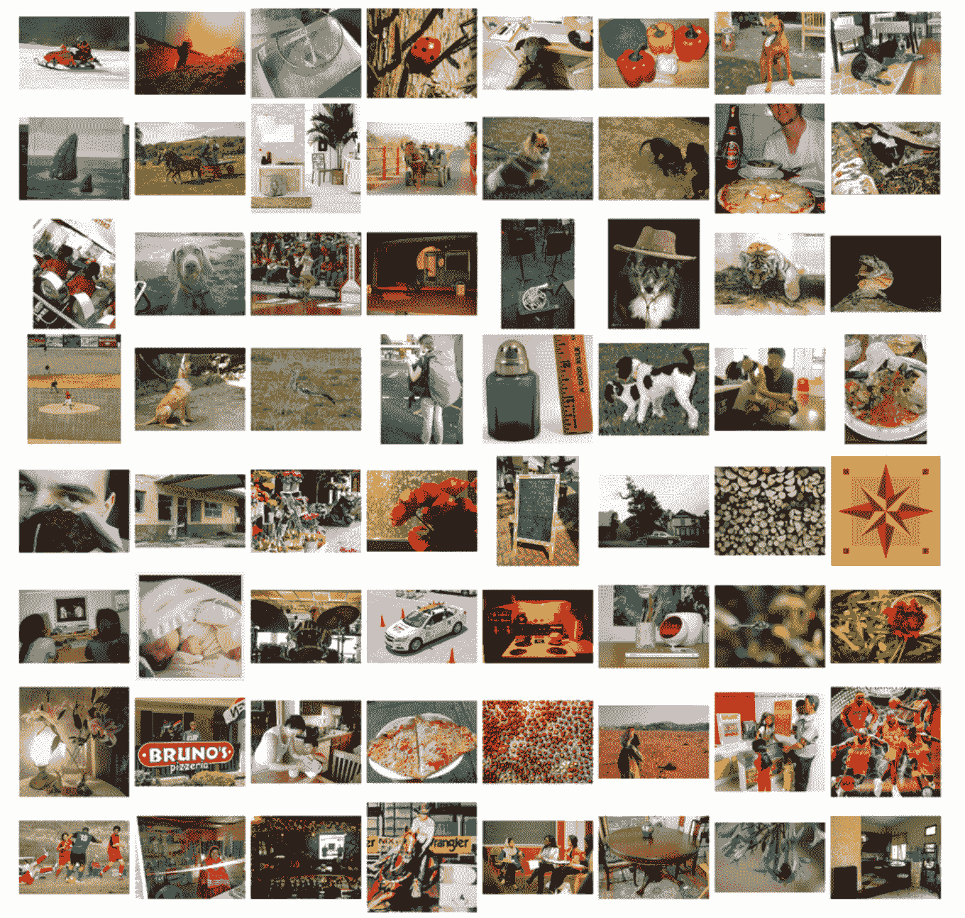
来自“ImageNet 大规模视觉识别挑战”的 ILSVRC 挑战
中使用的 ImageNet 数据集的图像样本,2015 年。
牛津 VGG 模型
来自牛津视觉几何组(简称 VGG)的研究人员参与了 ILSVRC 的挑战。
2014 年,由 VGG 开发的卷积神经网络模型(CNN)赢得了图像分类任务。
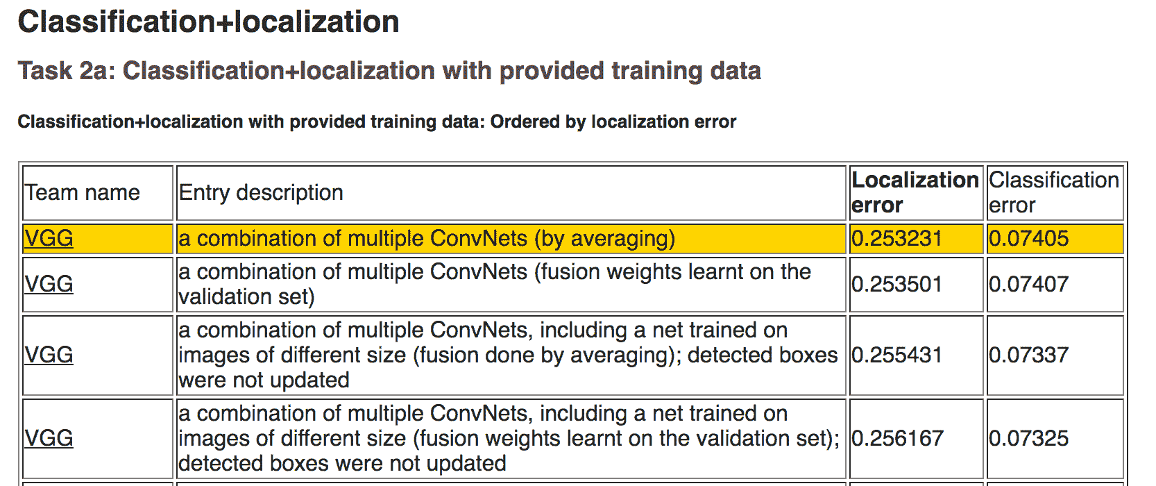
ILSVRC 2014 年的分类任务结果
比赛结束后,参与者在论文中写下了他们的发现:
- 用于大规模图像识别的非常深的卷积网络,2014 年。
这使得其他研究人员和开发人员可以在自己的工作和程序中使用最先进的图像分类模型。
这有助于推动一系列转移学习工作,其中使用预先训练的模型,对全新的预测性建模任务进行微小修改,利用经过验证的模型的最先进的特征提取功能。
…我们提出了更加精确的 ConvNet 架构,它不仅可以实现 ILSVRC 分类和定位任务的最先进精度,而且还适用于其他图像识别数据集,即使在用作相对简单的管道的一部分(例如,由线性 SVM 分类的深度特征,没有微调)。我们发布了两个表现最佳的模型,以促进进一步的研究。
- 用于大规模图像识别的非常深的卷积网络,2014 年。
VGG 发布了两种不同的 CNN 模型,特别是 16 层模型和 19 层模型。
有关这些型号的完整详细信息,请参阅本文。
VGG 模型不再仅仅是几个百分点的最新技术。然而,它们是非常强大的模型,既可用作图像分类器,也可用作使用图像输入的新模型的基础。
在下一节中,我们将看到如何在 Keras 中直接使用 VGG 模型。
在 Keras 中加载 VGG 模型
可以在 Keras 深度学习库中加载和使用 VGG 模型。
Keras 提供应用程序界面,用于加载和使用预先训练的模型。
使用此界面,您可以使用 Oxford 组提供的预训练权重创建 VGG 模型,并将其用作您自己模型中的起点,或者将其用作模型直接用于分类图像。
在本教程中,我们将重点介绍使用 VGG 模型对新图像进行分类的用例。
Keras 通过 VGG16 和 VGG19 类提供 16 层和 19 层版本。让我们关注 VGG16 模型。
可以按如下方式创建模型:
from keras.applications.vgg16 import VGG16
model = VGG16()
而已。
第一次运行此示例时,Keras 将从 Internet 下载权重文件并将其存储在 〜/ .keras / models 目录中。
注意权重约为 528 兆字节,因此下载可能需要几分钟,具体取决于您的 Internet 连接速度。
权重仅下载一次。下次运行示例时,权重将在本地加载,模型应该可以在几秒钟内使用。
我们可以使用标准的 Keras 工具来检查模型结构。
例如,您可以打印网络层的摘要,如下所示:
from keras.applications.vgg16 import VGG16
model = VGG16()
print(model.summary())
你可以看到模型很大。
您还可以看到,默认情况下,模型要求图像作为输入,大小为 224 x 224 像素,具有 3 个通道(例如颜色)。
_________________________________________________________________
Layer (type)                 Output Shape              Param #
=================================================================
input_1 (InputLayer)         (None, 224, 224, 3)       0
_________________________________________________________________
block1_conv1 (Conv2D)        (None, 224, 224, 64)      1792
_________________________________________________________________
block1_conv2 (Conv2D)        (None, 224, 224, 64)      36928
_________________________________________________________________
block1_pool (MaxPooling2D)   (None, 112, 112, 64)      0
_________________________________________________________________
block2_conv1 (Conv2D)        (None, 112, 112, 128)     73856
_________________________________________________________________
block2_conv2 (Conv2D)        (None, 112, 112, 128)     147584
_________________________________________________________________
block2_pool (MaxPooling2D)   (None, 56, 56, 128)       0
_________________________________________________________________
block3_conv1 (Conv2D)        (None, 56, 56, 256)       295168
_________________________________________________________________
block3_conv2 (Conv2D)        (None, 56, 56, 256)       590080
_________________________________________________________________
block3_conv3 (Conv2D)        (None, 56, 56, 256)       590080
_________________________________________________________________
block3_pool (MaxPooling2D)   (None, 28, 28, 256)       0
_________________________________________________________________
block4_conv1 (Conv2D)        (None, 28, 28, 512)       1180160
_________________________________________________________________
block4_conv2 (Conv2D)        (None, 28, 28, 512)       2359808
_________________________________________________________________
block4_conv3 (Conv2D)        (None, 28, 28, 512)       2359808
_________________________________________________________________
block4_pool (MaxPooling2D)   (None, 14, 14, 512)       0
_________________________________________________________________
block5_conv1 (Conv2D)        (None, 14, 14, 512)       2359808
_________________________________________________________________
block5_conv2 (Conv2D)        (None, 14, 14, 512)       2359808
_________________________________________________________________
block5_conv3 (Conv2D)        (None, 14, 14, 512)       2359808
_________________________________________________________________
block5_pool (MaxPooling2D)   (None, 7, 7, 512)         0
_________________________________________________________________
flatten (Flatten)            (None, 25088)             0
_________________________________________________________________
fc1 (Dense)                  (None, 4096)              102764544
_________________________________________________________________
fc2 (Dense)                  (None, 4096)              16781312
_________________________________________________________________
predictions (Dense)          (None, 1000)              4097000
=================================================================
Total params: 138,357,544
Trainable params: 138,357,544
Non-trainable params: 0
_________________________________________________________________
我们还可以在 VGG 模型中创建层,如下所示:
from keras.applications.vgg16 import VGG16
from keras.utils.vis_utils import plot_model
model = VGG16()
plot_model(model, to_file='vgg.png')
同样,因为模型很大,情节有点太大,也许不可读。然而,它在下面提供。
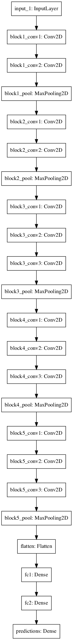
VGG 模型中的层图
VGG()类需要一些参数,如果您希望在自己的项目中使用该模型,可能只会感兴趣。转学习。
例如:
- include_top (
True):是否包含模型的输出层。如果您根据自己的问题拟合模型,则不需要这些。 - 权重(‘
imagenet’):要加载的权重。如果您有兴趣从零开始训练模型,则可以指定“无”以不加载预先训练的权重。 - input_tensor (_ 无 _):如果您打算在不同大小的新数据上拟合模型,则为新输入层。
- input_shape (_ 无 _):如果更改输入层,模型应采用的图像大小。
- 汇集(_ 无 _):训练一组新输出层时要使用的池类型。
- 类(
1000):模型的类数(例如输出向量的大小)。
接下来,让我们看一下使用加载的 VGG 模型对特定照片进行分类。
开发简单的照片分类器
让我们开发一个简单的图像分类脚本。
1.获取样本图像
首先,我们需要一个可以分类的图像。
你可以在这里从 Flickr 下载咖啡杯的随机照片。

咖啡杯
摄影: jfanaian ,保留一些权利。
下载图像并将其保存到当前工作目录,文件名为“mug.png”。
2.加载 VGG 模型
加载 VGG-16 型号的重量,就像我们在上一节中所做的那样。
from keras.applications.vgg16 import VGG16
# load the model
model = VGG16()
3.加载并准备图像
接下来,我们可以将图像作为像素数据加载并准备将其呈现给网络。
Keras 提供了一些帮助完成此步骤的工具。
首先,我们可以使用load_img()函数加载图像并将其大小调整为所需的 224×224 像素大小。
from keras.preprocessing.image import load_img
# load an image from file
image = load_img('mug.png', target_size=(224, 224))
接下来,我们可以将像素转换为 NumPy 数组,以便我们可以在 Keras 中使用它。我们可以使用img_to_array()函数。
from keras.preprocessing.image import img_to_array
# convert the image pixels to a numpy array
image = img_to_array(image)
网络期望一个或多个图像作为输入;这意味着输入数组需要是 4 维的:样本,行,列和通道。
我们只有一个样本(一个图像)。我们可以通过调用reshape()并添加额外的维度来重新整形数组。
# reshape data for the model
image = image.reshape((1, image.shape[0], image.shape[1], image.shape[2]))
接下来,需要以与准备 ImageNet 训练数据相同的方式准备图像像素。具体来说,从论文:
我们唯一的预处理是从每个像素中减去在训练集上计算的平均 RGB 值。
- 用于大规模图像识别的非常深的卷积网络,2014 年。
Keras 提供了一个名为preprocess_input()的函数来为网络准备新的输入。
from keras.applications.vgg16 import preprocess_input
# prepare the image for the VGG model
image = preprocess_input(image)
我们现在准备对我们加载和准备好的图像做出预测。
4.做出预测
我们可以在模型上调用predict()函数,以便预测属于 1000 种已知对象类型中的每一种的图像的概率。
# predict the probability across all output classes
yhat = model.predict(image)
几乎在那里,现在我们需要解释概率。
5.解释预测
Keras 提供了解释称为decode_predictions()的概率的函数。
它可以返回类列表及其概率,以防您想要呈现照片中可能存在的前 3 个对象。
我们将报告第一个最可能的对象。
from keras.applications.vgg16 import decode_predictions
# convert the probabilities to class labels
label = decode_predictions(yhat)
# retrieve the most likely result, e.g. highest probability
label = label[0][0]
# print the classification
print('%s (%.2f%%)' % (label[1], label[2]*100))
就是这样。
完整的例子
将所有这些结合在一起,下面列出了完整的示例:
from keras.preprocessing.image import load_img
from keras.preprocessing.image import img_to_array
from keras.applications.vgg16 import preprocess_input
from keras.applications.vgg16 import decode_predictions
from keras.applications.vgg16 import VGG16
# load the model
model = VGG16()
# load an image from file
image = load_img('mug.png', target_size=(224, 224))
# convert the image pixels to a numpy array
image = img_to_array(image)
# reshape data for the model
image = image.reshape((1, image.shape[0], image.shape[1], image.shape[2]))
# prepare the image for the VGG model
image = preprocess_input(image)
# predict the probability across all output classes
yhat = model.predict(image)
# convert the probabilities to class labels
label = decode_predictions(yhat)
# retrieve the most likely result, e.g. highest probability
label = label[0][0]
# print the classification
print('%s (%.2f%%)' % (label[1], label[2]*100))
运行该示例,我们可以看到图像被正确分类为“_ 咖啡杯 _”,可能性为 75%。
coffee_mug (75.27%)
扩展
本节列出了一些扩展您可能希望探索的教程的想法。
- 创建一个函数。更新示例并添加一个给定图像文件名的函数,加载的模型将返回分类结果。
- 命令行工具。更新示例,以便在命令行上给出图像文件名,程序将报告图像的分类。
- 报告多个类。更新示例以报告给定图像的前 5 个最可能的类及其概率。
进一步阅读
如果您要深入了解,本节将提供有关该主题的更多资源。
- ImageNet
- 维基百科上的 ImageNet
- 用于大规模图像识别的非常深的卷积网络,2015 年。
- 用于大规模视觉识别的非常深的卷积网络,位于牛津大学。
- 使用非常少的数据建立强大的图像分类模型,2016。
- Keras Applications API
- Keras 重量文件
摘要
在本教程中,您发现了用于图像分类的 VGG 卷积神经网络模型。
具体来说,你学到了:
- 关于 ImageNet 数据集和竞争以及 VGG 获奖模型。
- 如何在 Keras 中加载 VGG 模型并总结其结构。
- 如何使用加载的 VGG 模型对特定照片中的对象进行分类。
你有任何问题吗?
在下面的评论中提出您的问题,我会尽力回答。


 被折叠的 条评论
为什么被折叠?
被折叠的 条评论
为什么被折叠?
 到【灌水乐园】发言


