


Mann-Kendall原理
Mann-Kendall检验是一种用于检测时间序列中趋势变化的非参数统计方法,它不需要对数据分布做出任何假设,因此适用于各种类型的数据。
Mann-Kendall检验的假设是原假设:时间序列中不存在趋势变化,备择假设:时间序列中存在趋势变化。其基本思想是通过比较每对数据点之间的大小关系来检查序列中的趋势,然后根据秩和的正负性来确定趋势的方向。
Mann-Kendall检验的计算过程包括以下步骤:
1.对于长度为n的时间序列X,计算n(n-1)/2个变量关系差(d):
2.将所有d[i,j]的符号相乘,得到Sgn。即:
3.计算所有d[i,j]的绝对值的秩和,即:
4.计算标准正态分布的z统计量,即:
5.根据显著性水平选择拒绝原假设的临界值,如果z值小于临界值,则接受原假设,否则拒绝原假设。
在Mann-Kendall检验确定存在趋势后,可以使用Sen's slope来计算趋势的斜率。Sen's slope是一种计算趋势斜率的方法,它利用中位数差来估计趋势的斜率,与线性回归方法不同,Sen's slope不受异常值的影响,因此更适用于含有异常值的数据。
Sen's slope的计算方法如下:
1.对于长度为n的时间序列X,计算n(n-1)/2个变量关系差(d):
2.计算所有d[i,j]的绝对值的中位数,即:
3.计算Sen's slope,即:
其中,k = (n-1)/2
Sen's slope表示时间序列中单位时间的变化量。当Sen's slope为正数时,表示时间序列呈现上升趋势,当Sen's slope为负数时,表示时间序列呈现下降趋势。
简而言之,Sen's slope是所有点连线的中位数。
GEE JS
时间序列
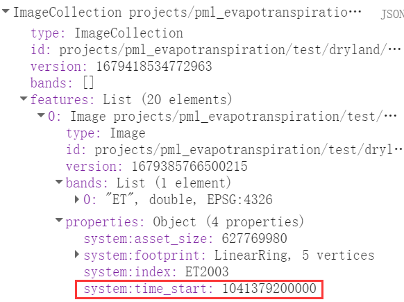
要求多年ImageCollection必须有时间属性:
以PML_v2的ET为例(也可也相应换成其它,如EVI、NDVI、LAI等等)
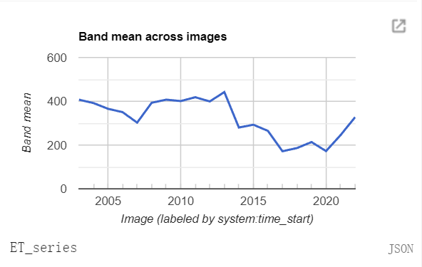
获取一个时间序列查看:
function get_chart(imgcol, name){


  var chart = ui.Chart.image.series({
      imageCollection: imgcol,
      region         : point,
      reducer        : ee.Reducer.mean(),
      scale          : 500
  });
  print(chart, name);
}

get_chart(img_ET.select('ET'), 'ET_series');
由于MK sensSlope的原理是所有时间连线的中位数
因此需要组成一个Join,构建了所有前后点的连线。施加一个Filter,使用lessThan过滤器将集合与其自身结合起来。过滤器将通过所有按时间顺序排列较晚的图像。在连接的集合中,每个图像都将在一个属性中存储它之后的所有图像after。
var afterFilter = ee.Filter.lessThan({
  leftField: 'system:time_start',
  rightField: 'system:time_start'
});
var coll = img_ET.select('ET')
var joined = ee.ImageCollection(ee.Join.saveAll('after').apply({
  primary: coll,
  secondary: coll,
  condition: afterFilter
}));
print(coll)
趋势检验
Mann-Kendall 趋势定义为所有正的符号之和。定义了sign函数,用来判断ET值大小(后减去前),正值为1,负值为 -1,相等为零。
var kendall = ee.ImageCollection(joined.map(function(current) {
  var afterCollection = ee.ImageCollection.fromImages(current.get('after'));
  return afterCollection.map(function(image) {
    // The unmask is to prevent accumulation of masked pixels that
    // result from the undefined case of when either current or image
    // is masked.  It won't affect the sum, since it's unmasked to zero.
    return ee.Image(sign(current, image)).unmask(0);
  });
  // Set parallelScale to avoid User memory limit exceeded.
}).flatten()).reduce('sum', 2);
var palette = ['red', 'white', 'green'];
// Stretch this as necessary.
Map.addLayer(kendall, {palette: palette}, 'kendall');
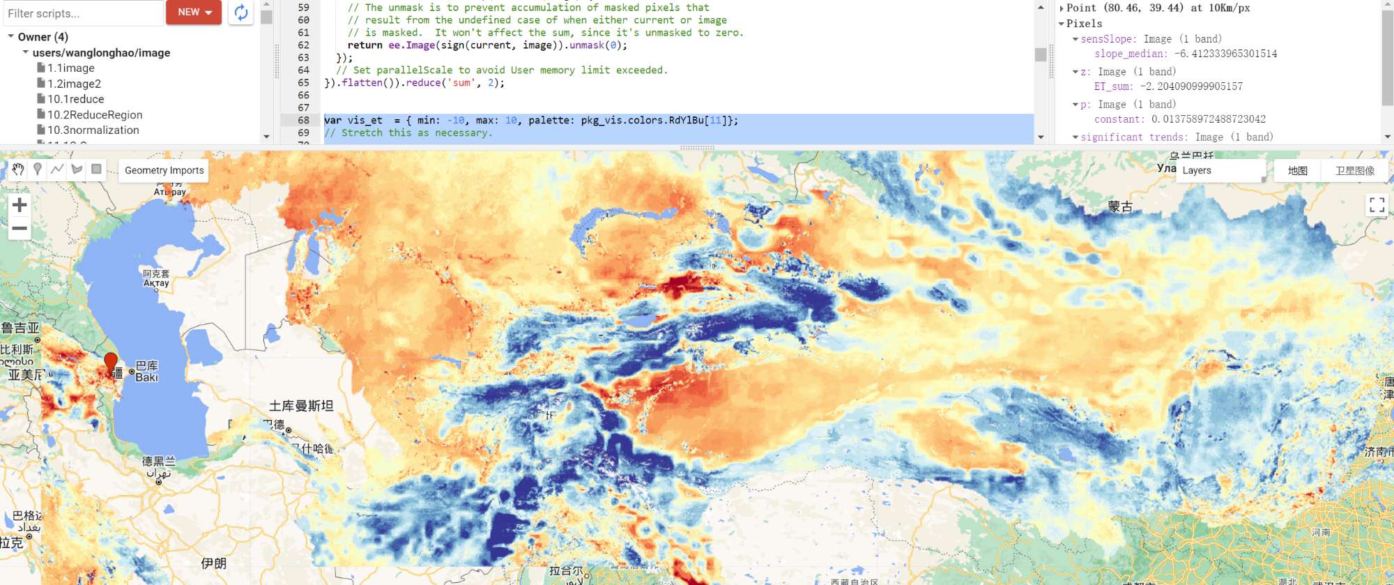
SensSlope
SensSlope的计算方式与 Mann-Kendall 统计量类似。但是,不是将所有正的符号相加,而是计算所有正sign的斜率。SensSlope是上述斜率中位数
尤其注意的是,我这里是年均值,ee.Date.difference是Year,如果是日序列改为days
var vis_et  = { min: -10, max: 10, palette: pkg_vis.colors.RdYlBu[11]};
// Stretch this as necessary.

var slope = function(i, j) { // i and j are images
  return ee.Image(j).subtract(i)
      .divide(ee.Image(j).date().difference(ee.Image(i).date(), 'year'))
      .rename('slope')
      .float();
};

var slopes = ee.ImageCollection(joined.map(function(current) {
  var afterCollection = ee.ImageCollection.fromImages(current.get('after'));
  return afterCollection.map(function(image) {
      return ee.Image(slope(current, image));
  });
}).flatten());

var sensSlope = slopes.reduce(ee.Reducer.median(), 2); // Set parallelScale.
Map.addLayer(sensSlope, vis_et, 'sensSlope');
计算方差
还记得原理中公式4的方差吗?
具体的推导请看Mann和Kendall两位学者于1945发表在Econometrica的《Nonparametric tests against trend》
(反正比较麻烦)

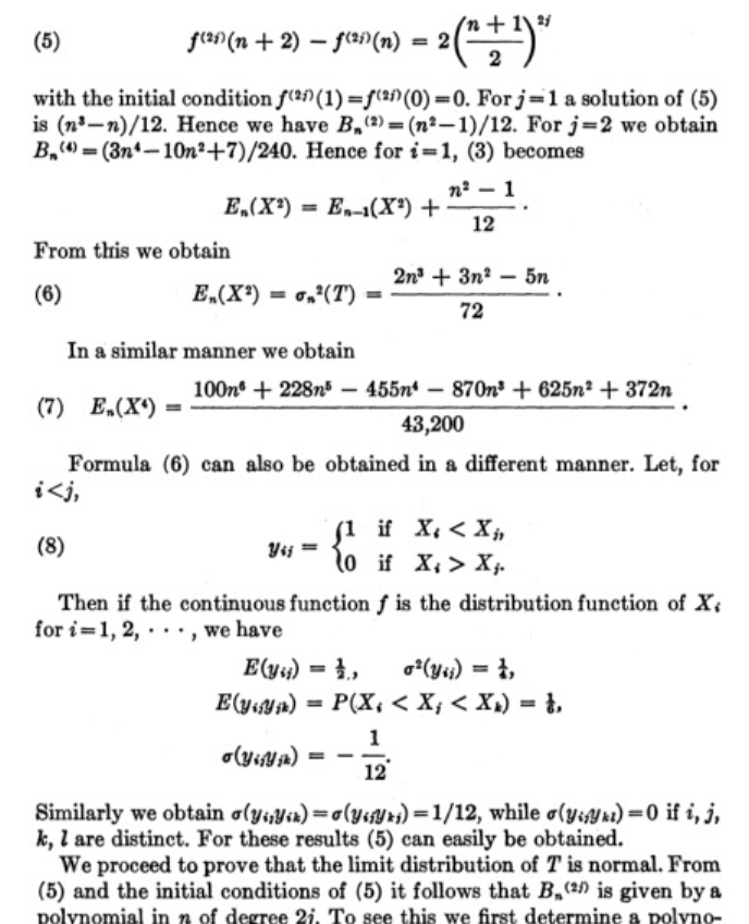
这里直接套公式:
// Values that are in a group (ties).  Set all else to zero.
var groups = coll.map(function(i) {
  var matches = coll.map(function(j) {
    return i.eq(j); // i and j are images.
  }).sum();
  return i.multiply(matches.gt(1));
});

// Compute tie group sizes in a sequence.  The first group is discarded.
var group = function(array) {
  var length = array.arrayLength(0);
  // Array of indices.  These are 1-indexed.
  var indices = ee.Image([1])
      .arrayRepeat(0, length)
      .arrayAccum(0, ee.Reducer.sum())
      .toArray(1);
  var sorted = array.arraySort();
  var left = sorted.arraySlice(0, 1);
  var right = sorted.arraySlice(0, 0, -1);
  // Indices of the end of runs.
  var mask = left.neq(right)
  // Always keep the last index, the end of the sequence.
      .arrayCat(ee.Image(ee.Array([[1]])), 0);
  var runIndices = indices.arrayMask(mask);
  // Subtract the indices to get run lengths.
  var groupSizes = runIndices.arraySlice(0, 1)
      .subtract(runIndices.arraySlice(0, 0, -1));
  return groupSizes;
};

// See equation 2.6 in Sen (1968).
var factors = function(image) {
  return image.expression('b() * (b() - 1) * (b() * 2 + 5)');
};

var groupSizes = group(groups.toArray());
var groupFactors = factors(groupSizes);
var groupFactorSum = groupFactors.arrayReduce('sum', [0])
      .arrayGet([0, 0]);

var count = joined.count();

var kendallVariance = factors(count)
    .subtract(groupFactorSum)
    .divide(18)
    .float();
//Map.addLayer(kendallVariance, {}, 'kendallVariance');
显著性检验
对于适当大的样本,Mann-Kendall 统计量渐近正态。
假设我们的样本足够大且不相关。在这些假设下,Mann-Kendall 统计量的真实均值为零,方差在上一步已经计算好了。
要计算标准正态统计量 ( z),请将统计量除以其标准差。z 统计量的 P 值为
对于在 95% 置信水平(双边检验)下检验存在正面或负面趋势的置信度。将 P 值与 0.95进行比较。
// Compute Z-statistics.
var zero = kendall.multiply(kendall.eq(0));
var pos = kendall.multiply(kendall.gt(0)).subtract(1);
var neg = kendall.multiply(kendall.lt(0)).add(1);
var z = zero
.add(pos.divide(kendallVariance.sqrt()))
.add(neg.divide(kendallVariance.sqrt()));
Map.addLayer(z, {min: -2, max: 2}, 'z');
// https://en.wikipedia.org/wiki/Error_function#Cumulative_distribution_function
function eeCdf(z) {
return ee.Image(0.5)
.multiply(ee.Image(1).add(ee.Image(z).divide(ee.Image(2).sqrt()).erf()));
}
function invCdf(p) {
return ee.Image(2).sqrt()
.multiply(ee.Image(p).multiply(2).subtract(1).erfInv());
}
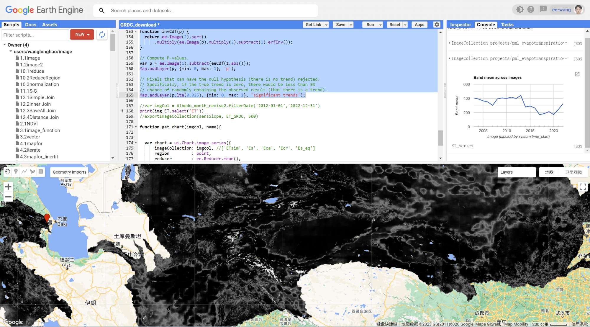
// Compute P-values.
var p = ee.Image(1).subtract(eeCdf(z.abs()));
Map.addLayer(p, {min: 0, max: 1}, 'p');
// Pixels that can have the null hypothesis (there is no trend) rejected.
// Specifically, if the true trend is zero, there would be less than 5%
// chance of randomly obtaining the observed result (that there is a trend).
Map.addLayer(p.lte(0.05), {min: 0, max: 1}, 'significant trends');
计算的P值如下:
Python API
对于python API只要将上述函数重写为python就可以了:
以NDVI为例,使用geemap:
计算NDVI
加载中国边界
countries = geemap.shp_to_ee("../data/countries.shp")
roi = countries.filterMetadata('NAME','equals', 'China')
计算NDVI
这里是定义了两个函数maskcloud和ndvi
然后使用List循环计算每年的NDVI,再后续进行MK检验
这里尤其注意的是通过setMulti添加Year属性,便于后续计算sensSlope
# 去云操作

def maskcloud(image):
    qa = image.select('BQA')
    mask = qa.bitwiseAnd(1 << 4).Or(qa.bitwiseAnd(1 << 8))
    return image.updateMask(mask.Not())
# 计算NDVI
def ndvi(image):
    ndvi = image.normalizedDifference(['B5', 'B4']).rename('NDVI')
    return image.addBands(ndvi)


time = ee.List.sequence(2013, 2020)
def funyear(year):
    year_origin = year
    year = ee.Number(year).format("%04d").cat('-01-01')
    image = ee.ImageCollection("LANDSAT/LC08/C01/T1_RT_TOA")\
    .filterBounds(roi)\
    .filterDate(year, ee.Date(year).advance(1, 'year'))\
    .map(maskcloud)\
    .map(ndvi)\
    .median()\
    .select(['NDVI'])\
    .clip(roi.geometry())\
    .setMulti({'system:index':year, 'system:time_start':ee.Date(year), 'year':ee.Number(year_origin)})
    return image

imgYear = time.map(funyear)
imgYear = ee.ImageCollection(imgYear)
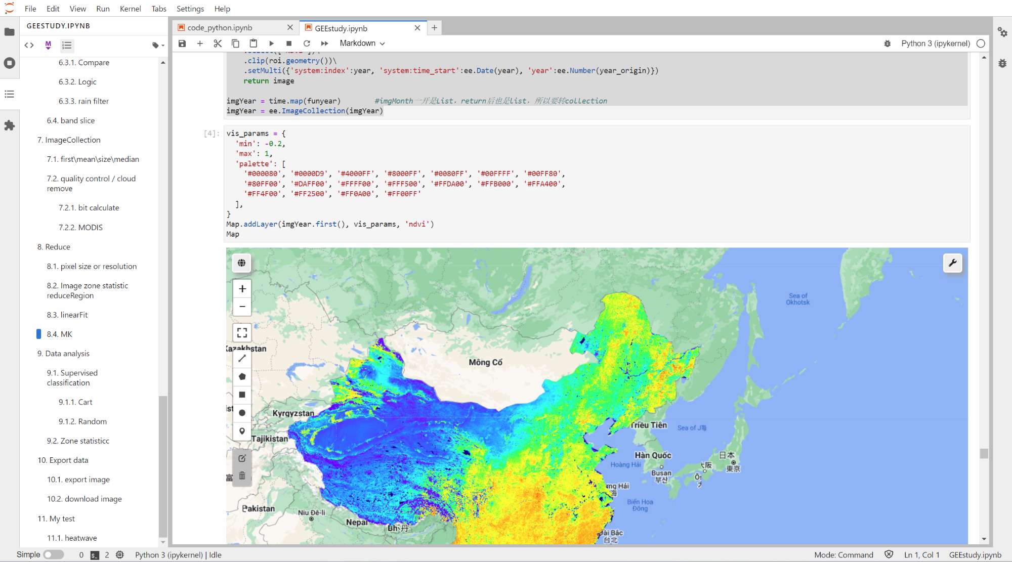
加载可视化:
vis_params = {
  'min': -0.2,
  'max': 1,
  'palette': [
    '#000080', '#0000D9', '#4000FF', '#8000FF', '#0080FF', '#00FFFF', '#00FF80',
    '#80FF00', '#DAFF00', '#FFFF00', '#FFF500', '#FFDA00', '#FFB000', '#FFA400',
    '#FF4F00', '#FF2500', '#FF0A00', '#FF00FF'
  ],
}
Map.addLayer(imgYear.first(), vis_params, 'ndvi')
Map
MK检验
进行MK检验,首先需要组成一个Join,构建了所有前后点的连线。
注意这里的Field是之前手动添加的'year'属性
afterFilter = ee.Filter.lessThan(
    leftField = 'year',
    rightField = 'year'
)

joined = ee.ImageCollection(ee.Join.saveAll('after').apply(
    primary = imgYear,
    secondary = imgYear,
    condition = afterFilter
))
之后定义两个函数,与之前JS相同,只是定义函数的方式不一样,python是def
def sign(i, j):  # i and j are images:
    return ee.Image(j).neq(i).multiply(ee.Image(j).subtract(i).clamp(-1, 1)).int()

def func(current):
    afterCollection = ee.ImageCollection.fromImages(current.get('after'))
    return afterCollection.map(lambda image: ee.Image(sign(current, image)).unmask(0))

kendall = ee.ImageCollection(joined.map(func).flatten()).sum()

#palette = ['red', 'yellow', 'green'];
#Map.addLayer(kendall, {'min':-100,'max':100, 'palette': palette}, 'kendall')
计算SensSlope
计算sensSlope并可视化
相对于传统的JS定义函数.map(function(img){}),python则要改写为匿名函数lambda img: img...
def slope(i, j):
# return ee.Image(j).subtract(i).divide(ee.Image(j).date().difference(ee.Image(i).date(), 'days')).rename('slope').float()
return ee.Image(j).subtract(i).divide(ee.Number(ee.Image(j).get('year')).subtract(ee.Number(ee.Image(i).get('year')))).rename('slope').float()
slopes = ee.ImageCollection(joined.map(lambda current: ee.ImageCollection.fromImages(current.get('after'))\
.map(lambda image: ee.Image(slope(current, image)))).flatten())
sensSlope = slopes.reduce(ee.Reducer.median(), 2)
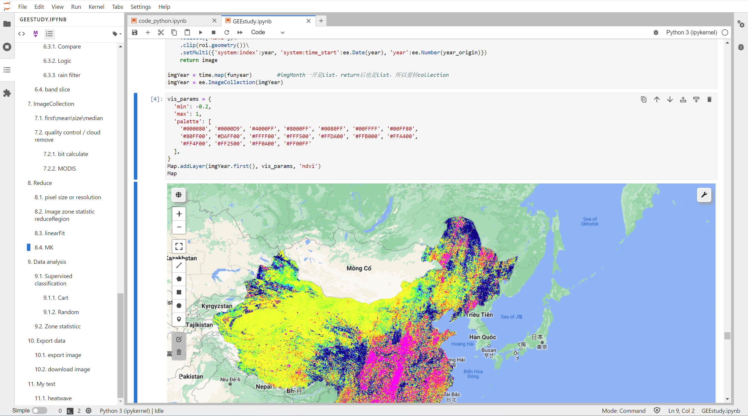
vis_params = {
'min': -0.01,
'max': 0.01,
'palette': [
'#000080', '#0000D9', '#4000FF', '#8000FF', '#0080FF', '#00FFFF', '#00FF80',
'#80FF00', '#DAFF00', '#FFFF00', '#FFF500', '#FFDA00', '#FFB000', '#FFA400',
'#FF4F00', '#FF2500', '#FF0A00', '#FF00FF'
],
}
Map.addLayer(sensSlope, vis_params, 'sensSlope')
#Map
计算方差和显著性检验
与JS相同,直接改写形式即可:
## image
groups = imgYear.map(lambda i: i.multiply(imgYear.map(lambda j: i.eq(j)).sum().gt(1)))
##
def group(array):
    length = array.arrayLength(0)
    indices = ee.Image([1]).arrayRepeat(0, length).arrayAccum(0, ee.Reducer.sum()).toArray(1)
    sorted = array.arraySort()
    left = sorted.arraySlice(0, 1)
    right = sorted.arraySlice(0, 0, -1)
    mask = left.neq(right).arrayCat(ee.Image(ee.Array([[1]])), 0)
    runIndices = indices.arrayMask(mask)
    groupSizes = runIndices.arraySlice(0, 1).subtract(runIndices.arraySlice(0, 0, -1))
    return groupSizes

def factors(image):
    return image.expression('b() * (b() - 1) * (b() * 2 + 5)')


groupSizes = group(groups.toArray())
groupFactors = factors(groupSizes)
groupFactorSum = groupFactors.arrayReduce('sum', [0]).arrayGet([0, 0])

count = joined.count()

kendallVariance = factors(count).subtract(groupFactorSum).divide(18).float()
#Map.addLayer(kendallVariance, {}, 'kendallVariance')
zero = kendall.multiply(kendall.eq(0));
pos = kendall.multiply(kendall.gt(0)).subtract(1);
neg = kendall.multiply(kendall.lt(0)).add(1);

z = zero.add(pos.divide(kendallVariance.sqrt())).add(neg.divide(kendallVariance.sqrt()))
#Map.addLayer(z, {'min': -2, 'max': 2}, 'z');

def eeCdf(z):
    return ee.Image(0.5).multiply(ee.Image(1).add(ee.Image(z).divide(ee.Image(2).sqrt()).erf()))

def invCdf(p):
    ee.Image(2).sqrt().multiply(ee.Image(p).multiply(2).subtract(1).erfInv())

# Compute P-values.
p = ee.Image(1).subtract(eeCdf(z.abs()))
Map.addLayer(p, {'min': 0, 'max': 1}, 'p')

#Map.addLayer(p.lte(0.025), {min: 0, max: 1}, 'significant trends')
#Map
Highlights
-
本文介绍了Mann-Kendall的原理 -
分Javascript和python两种接口下进行了实现 -
介绍了python API不同于Javascript的一些操作和改写方法
参考
[1] Mann, H. B. (1945). NONPARAMETRIC TESTS AGAINST TREND. Econometrica, 13(3), 245-259. https://doi.org/10.2307/1907187
[2] Non-Parametric Trend Analysis, Google Earth Engine Community. https://developers.google.cn/earth-engine/tutorials/community/nonparametric-trends
本文由 mdnice 多平台发布


 4793
4793

 被折叠的 条评论
为什么被折叠?
被折叠的 条评论
为什么被折叠?
 到【灌水乐园】发言


