TensorFlow学习（一）: 构建卷积神经网络

最新推荐文章于 2024-09-17 20:23:23 发布

iTensor

最新推荐文章于 2024-09-17 20:23:23 发布

阅读量2.5k

点赞数

分类专栏： TensorFlow 深度学习文章标签： TensorFlow 深度学习

深度学习同时被 2 个专栏收录

17 篇文章 0 订阅

订阅专栏

TensorFlow

8 篇文章 0 订阅

订阅专栏

欢迎点击参观我的 ——> 个人学习网站
TensorFlow的 layers 模块提供了一个高级API，可以轻松构建神经网络。它提供了便于创建全连接层和卷积层的方法，添加了激活函数以及应用DropOut正则化(防止过拟合)。在本教程中，您将学习如何构建卷积神经网络模型来识别MNIST数据集中的手写数字。
这里写图片描述

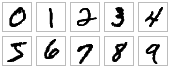
MNIST数据集包含60,000个训练样例和10,000个手写数字0-9的测试示例，格式为28x28像素单色图像。

完整代码已上传至github。

开始

首先写出TensorFlow程序的基本框架。创建 cnn_mnist.py ，添加下面的代码：

import numpy as np
import tensorflow as tf

tf.logging.set_verbosity(tf.logging.INFO)

if __name__ == "__main__":
  tf.app.run()

如果用的python2，请在最上面添加：

from __future__ import absolute_import
from __future__ import division
from __future__ import print_function

CNNs（卷及神经网络）简介

个人觉得以下能理解尽量理解，不能理解的话可以简单参考”数字图像处理“。实在不能理解，知道卷积核如何运算到数据上也可以，因为接下来的操作都是数学坑了。

卷积神经网络（CNN）是当前用于图像分类任务的最先进的模型。CNN将一系列滤波器（卷积核）应用于图像的原始像素数据以提取和学习更高级别的特征，然后该模型可用于分类。 CNN包含三个组件：

下面属博主个人理解，和官网有些差异。可参考TensorFlow官网。

卷积层: 用人工事先定义好的卷积核对图像进行卷积计算，输出采用ReLU激活函数。对于本代码的补0卷积计算，可参考下图：
这里写图片描述
池化层: 简单来说就是对卷积过后的特征进行下采样，也就是减少图像的空间大小。通常使用max-pooling，既在规定的窗口大小下取最大。例如定义2×2的尺寸，池化后：

输出层: 经过卷积和池化的运算，特征提取完毕。再通过输出层计算输出可知道样本所属的类别了。一般输出层采用 softmax 激活函数，产生结果为属于某类别的概率，所有结果加起来总和为1。

整个过程可看下图简单理解：

这里写图片描述

构建CNN的MNIST分类器

让我们构建一个模型，使用以下CNN结构对MNIST数据集中的图像进行分类：
1. 卷积层1： 使用32 5×5的卷积核，ReLU激活函数。
2. 池化层1： 使用步长为2，尺寸为2×2的窗口。
3. 卷积层2： 使用64 5×5的卷积核，ReLU激活函数。
4. 池化层2： 使用步长为2，尺寸为2×2的窗口。
5. 特征处理层： 1024个节点。在训练中，DropOut正则率为0.4（任何给定的特征在训练中都会以0.4的概率被丢弃）（知道用来防止过拟合即可）
6. 输出层： 10个节点，输出0-9各自的概率，例如8的概率最大，即表示图像的数字是 8。

tf.layers 模块包含了创建上面各种层的方法：

conv2d() 构造一个二维卷积层。需要卷积核数量,卷积核大小,是否填充和激活函数作为参数。
max_pooling2d() 使用max-pooling构造一个二维的池层。将池化窗口大小和步长作为参数
dense() 构造一个全连接层。以神经元节点数和激活函数为参数。

定义cnn_model_fn函数。将MNIST的特征、标签和模型模式（TRAIN、EVAL、PREDICT）作为参数；并返回预测、损失和训练记录。

def cnn_model_fn(features, labels, mode)

输入层

输入数据向量的格式为 [batch_size, image_width, image_height, channels] 定义如下：

batch_size: 在训练梯度下降时每次训练的样本个数。
image_width: 图像训练样本的宽度。
image_height: 图像训练样本的高度。
channels: 图像样本中的颜色通道数量，彩色图像一般是3个通道（红、绿、蓝），而黑白图像只有单个通道（黑）。

MNIST数据集是由单通道[28×28]像素组成的图像集。

input_layer = tf.reshape(features["x"], [-1, 28, 28, 1])

定义 batch_size =1，指定了这个维度应该根据输入值的数量动态计算features(“x”)，保持所有其他维度的大小不变。详见这里。

卷积层1

conv1 = tf.layers.conv2d(
      inputs=input_layer, 
      filters=32, 
      kernal_size=[5, 5], 
      padding='same', 
      activation=tf.nn.relu)

注： padding 参数有两种：valid 和 same。 same 是在卷积后填0，使得得到的特征尺寸大小和输入时的大小一样，而 valid 则是默认，28x28运算后得到的是24x24。
经conv2d() 后的形状是 [batch_size, 28, 28, 32]

池化层1

pool1 = tf.layers.max_pooling2d(
      inputs=conv1, 
      pool_size=[2, 2], 
      strides=2)

经过 max_pooling2d() 后得到的形状大小为 [batch_size, 14, 14, 32] 。

卷积层2

conv2 = tf.layers.conv2d(
      inputs=pool1, 
      filters=64, 
      kernal_size=[5, 5], 
      padding='same', 
      activation=tf.nn.relu)

池化层2

pool2 = tf.layers.max_pooling2d(
      inputs=conv2, 
      pool_size=[2, 2], 
      strides=2)

最后得到特征大小为 [batch_size, 7, 7, 64] 。

特征处理层

我们想要在CNN中添加一个全连接层（包含1,024个神经元节点和ReLU激活函数），以对由卷积/池化层提取的特征进行分类。

pool2_flat = tf.reshape(pool2, [-1, 7 * 7 * 64])
dense = tf.layers.dense(
    inputs=pool2_flat, 
    activation=tf.nn.relu)
dropout = tf.layers.dropout(
    inputs=dense, 
    rate=0.4, 
    training=mode ==tf.estimator.ModeKeys.TRAIN)

training参数采用布尔值来指定模型当前是否在训练模式下运行，当为True 时dropout 才运行。我们检查传递给函数cnn_model_fn的模式是否是TRAIN模式。
最后得到特征大小为 [batch_size, 1024] 。

输出层

logits = tf.layers.dense(inputs=dropout, units=10)

预测

讲预测类别和概率放入一个dict中，并返回一个EstimatorSpec对象。

if mode == tf.estimator.ModeKeys.PREDICT：
    return tf.estimator.EstimatorSpec(mode=mode, predictions=predictions)

计算损失

使用交叉熵

loss = tf.losses.sparse_softmax_cross_entropy(labels=labels, logits=logits)

训练

通过交叉熵得到损失后，设置0.001的学习率和SGD（随机梯度下降）算法，通过训练优化损失。

if mode == tf.estimator.ModeKeys.TRAIN:
    optimizer = tf.train.GradientDescentOptimizer(learing_rate=0.001)
    train_op = optimizer.minimize(loss=loss, global_step=tf.train.get_global_step())
    return tf.estimator.EstimatorSpec(mode=mode, loss=loss, train_op=train_op)

评估指标

eval_metric_ops = {
      "accuracy": tf.metrics.accuracy(
          labels=labels, predictions=predictions["classes"])
      return tf.estimator.EstimatorSpec(
          mode=mode, loss=loss, eval_metric_ops=eval_metric_ops)}

训练和评估CNN分类器

定义main()函数

加载数据

def main(unused_argv):
  mnist = tf.contrib.learn.datasets.load_dataset("mnist")
  train_data = mnist.train.images # Returns np.array
  train_labels = np.asarray(mnist.train.labels, dtype=np.int32)
  eval_data = mnist.test.images # Returns np.array
  eval_labels = np.asarray(mnist.test.labels, dtype=np.int32)

构建Estimator

mnist_classifier = tf.estimator.Estimator(
      model_fn=cnn_model_fn, model_dir="/tmp/mnist_convnet_model")

设置Logging Hook

由于CNN可能需要一段时间才能进行训练，因此我们设置一些日志记录，以便在训练期间跟踪进度。

tensors_to_log = {"probabilities": "softmax_tensor"}
  logging_hook = tf.train.LoggingTensorHook(
      tensors=tensors_to_log, every_n_iter=50)

训练模型

train_input_fn = tf.estimator.inputs.numpy_input_fn(
      x={"x": train_data}, 
      y=train_labels, 
      batch_size=100, 
      num_epochs=None, 
      shuffle=True) 
  mnist_classifier.train(
      input_fn=train_input_fn,
      steps=20000,
      hooks=[logging_hook])

输入x必须是dict型； batch_size=100即小批量梯度下降每次训练的样本数为100；
num_epochs=None即模型一直运行完设置的steps=20000时停止；
shuffle=True即训练时样本是随机抽取的

评估模型

eval_input_fn = tf.estimator.inputs.numpy_input_fn(
    x={"x": eval_data},
    y=eval_labels,
    num_epochs=1,
    shuffle=False)
eval_results = mnist_classifier.evaluate(input_fn=eval_input_fn)
print(eval_results)

运行结果

Extracting MNIST-data/train-images-idx3-ubyte.gz
Extracting MNIST-data/train-labels-idx1-ubyte.gz
Extracting MNIST-data/t10k-images-idx3-ubyte.gz
Extracting MNIST-data/t10k-labels-idx1-ubyte.gz
INFO:tensorflow:Using default config.
INFO:tensorflow:Using config: {'_model_dir': '/tmp/mnist_convnet_model', '_tf_random_seed': None, '_save_summary_steps': 100, '_save_checkpoints_steps': None, '_save_checkpoints_secs': 600, '_session_config': None, '_keep_checkpoint_max': 5, '_keep_checkpoint_every_n_hours': 10000, '_log_step_count_steps': 100, '_service': None, '_cluster_spec': <tensorflow.python.training.server_lib.ClusterSpec object at 0x7f35eb339128>, '_task_type': 'worker', '_task_id': 0, '_global_id_in_cluster': 0, '_master': '', '_evaluation_master': '', '_is_chief': True, '_num_ps_replicas': 0, '_num_worker_replicas': 1}
INFO:tensorflow:Calling model_fn.
INFO:tensorflow:Done calling model_fn.
INFO:tensorflow:Create CheckpointSaverHook.
INFO:tensorflow:Graph was finalized.
INFO:tensorflow:Running local_init_op.
INFO:tensorflow:Done running local_init_op.
INFO:tensorflow:Saving checkpoints for 1 into /tmp/mnist_convnet_model/model.ckpt.
INFO:tensorflow:probabilities = [[0.10603123 0.11674101 0.09009421 0.09591874 0.09321657 0.0876532
  0.09703767 0.10731895 0.10852493 0.09746351]
 [0.12638797 0.09118222 0.09904857 0.08684804 0.09524325 0.09678999
  0.09612204 0.09447883 0.10238035 0.11151876]
 [0.10961667 0.09775148 0.09031133 0.09005759 0.09975118 0.09663537
  0.09558715 0.10681319 0.10184265 0.11163338]
 [0.10582132 0.08626121 0.09644306 0.09036049 0.09503932 0.09686131
  0.10292714 0.1105746  0.11193833 0.10377329]
 ......
 ......
 ......