LSTM-多变量-单时间步-pytorch-负荷预测（多时间步采用滚动预测）

问题描述

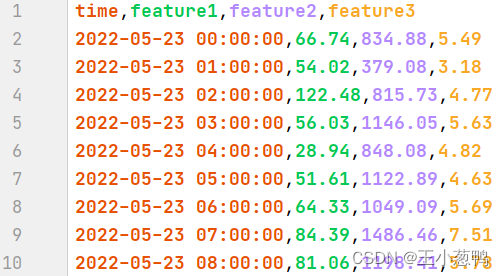
使用LSTM做负荷预测问题，数据共计456行，每一行3个特征，用过去N个时间段特征，预测未来第N+1个时间点的特征，数据格式如下，用00:00:00-04:00:00的[feature1，feature2，feature3]，预测第05:00:00的[feature1，feature2，feature3]。本问题属于多变量预测，输入是多变量-多时间步，输出也是多变量，只不过输出是一个时间点，可以使用循环的方式预测多个时间步。

模块导入

import pandas as pd
import matplotlib.pyplot as plt
import torch.nn as nn
import torch
import time
import numpy as np
import random

2 数据处理

2.1 数据导入以及可视化

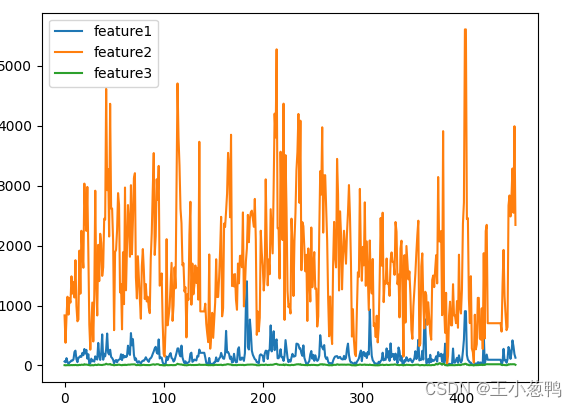
data = pd.read_csv("负荷-3变量.csv")
data.plot()
plt.show()

2.2 划分测试集和训练集

data = data.iloc[:, [1, 2, 3]].values  # 获取数值 456 *3
p = 48 # 预测未来48个小时的数据
train_data = data[:-p]
test_data = data[-p:]

• train_data 维度：408*3
• test_data 维度：48*3

2.3 数据归一化

每一列都需要单独归一化，所以axis的值为0

min_data = np.min(train_data, axis=0)
max_data = np.max(train_data, axis=0)
train_data_scaler = (train_data - min_data) / (max_data - min_data)

2.4 将一个序列划分为x和y

制作数据集，对应的x和y，假设用前12个时间步预测第13个时间点，则：

• x 维度：12 *3
• y 维度：1 *3
  假设用前24个时间步预测第25个时间点，则：
• x 维度：24 *3
• y 维度：1 *3

def get_x_y(data, step=12):
    # x : 12*3
    # y: 1 *3
    x_y = []
    for i in range(len(data) - step):
        x = data[i:i + step, :]
        y = np.expand_dims(data[i + step, :], 0)
        x_y.append([x, y])
    return x_y

2.5 生成mini_batch数据

假设batch_size = 16, 则生成的数据维度为：

• x:16* 12 * 3
• y: 16 * 1 * 3

def get_mini_batch(data, batch_size=16):
    # x: 16 * 12 *3
    # y :16 * 1 *3
    for i in range(0, len(data) - batch_size, batch_size):
        samples = data[i:i + batch_size]
        x, y = [], []
        for sample in samples:
            x.append(sample[0])
            y.append(sample[1])
        yield np.asarray(x), np.asarray(y)

3 模型搭建和训练

3.1 搭建模型

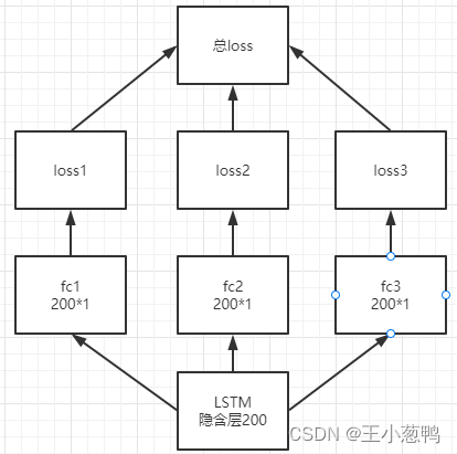
在处理多变量预测时，我们将lstm输出分别连接3个fc层，每个变量都单独计算loss，再把loss进行相加作为总的loss，示意图如下所示：

device = torch.device("cuda:0" if torch.cuda.is_available() else "cpu")
class LSTM(nn.Module):  # 注意Module首字母需要大写
    def __init__(self, hidden_size, num_layers, output_size, batch_size):
        super().__init__()
        self.hidden_size = hidden_size  # 隐含层神经元数目 100
        self.num_layers = num_layers  # 层数 通常设置为2
        self.output_size = output_size  # 48 一次预测下48个时间步
        self.num_directions = 1
        self.input_size = 3
        self.batch_size = batch_size
        # 初始化隐藏层数据
        self.hidden_cell = (
            torch.randn(self.num_directions * self.num_layers, self.batch_size, self.hidden_size).to(device),
            torch.randn(self.num_directions * self.num_layers, self.batch_size, self.hidden_size).to(device))

        self.lstm = nn.LSTM(self.input_size, self.hidden_size, self.num_layers, batch_first=True).to(device)
        self.fc1 = nn.Linear(self.hidden_size, self.output_size).to(device)
        self.fc2 = nn.Linear(self.hidden_size, self.output_size).to(device)
        self.fc3 = nn.Linear(self.hidden_size, self.output_size).to(device)

    def forward(self, input):
        output, _ = self.lstm(torch.FloatTensor(input).to(device), self.hidden_cell)
        pred1, pred2, pred3 = self.fc1(output), self.fc2(output), self.fc3(output)
        pred1, pred2, pred3 = pred1[:, -1, :], pred2[:, -1, :], pred3[:, -1, :]
        pred = torch.stack([pred1, pred2, pred3], dim=2)
        return pred

3.2 训练模型

epochs = 200
for i in range(epochs):
    start = time.time()
    for seq_batch, label_batch in get_mini_batch(train_x_y, batch_size):
        optimizer.zero_grad()
        y_pred = model(seq_batch)
        loss = 0
        for j in range(3):
            loss += loss_function(y_pred[:,:, j], torch.FloatTensor(label_batch[:, :, j]).to(device))
        loss /= 3
        loss.backward()  # 调用loss.backward()自动生成梯度，
        optimizer.step()  # 使用optimizer.step()执行优化器，把梯度传播回每个网络
        # 查看模型训练的结果
    print(f'epoch:{i:3} loss:{loss.item():10.8f} time:{time.time() - start:6}')

3.3 预测模型

model.eval()
with torch.no_grad():
   model.hidden_cell = (torch.zeros(1 * num_layers, 1, hidden_size).to(device),
                        torch.zeros(1 * num_layers, 1, hidden_size).to(device))
   # 测试集
   total_test_loss = 0
   test_pred = np.zeros(shape=(p, 3))
   for i in range(len(test_data)):
       x = train_data_scaler[-time_step:, :]
       x1 = np.expand_dims(x, 0)
       test_y_pred_scalar = np.expand_dims(model(x1).cpu().squeeze().numpy(), 0)  # 预测的值0-1
       train_data_scaler = np.append(train_data_scaler, test_y_pred_scalar, axis=0)
       y = test_y_pred_scalar * (max_data - min_data) + min_data
       test_pred[i,:] = y

   x_in = list(range(len(test_pred)))

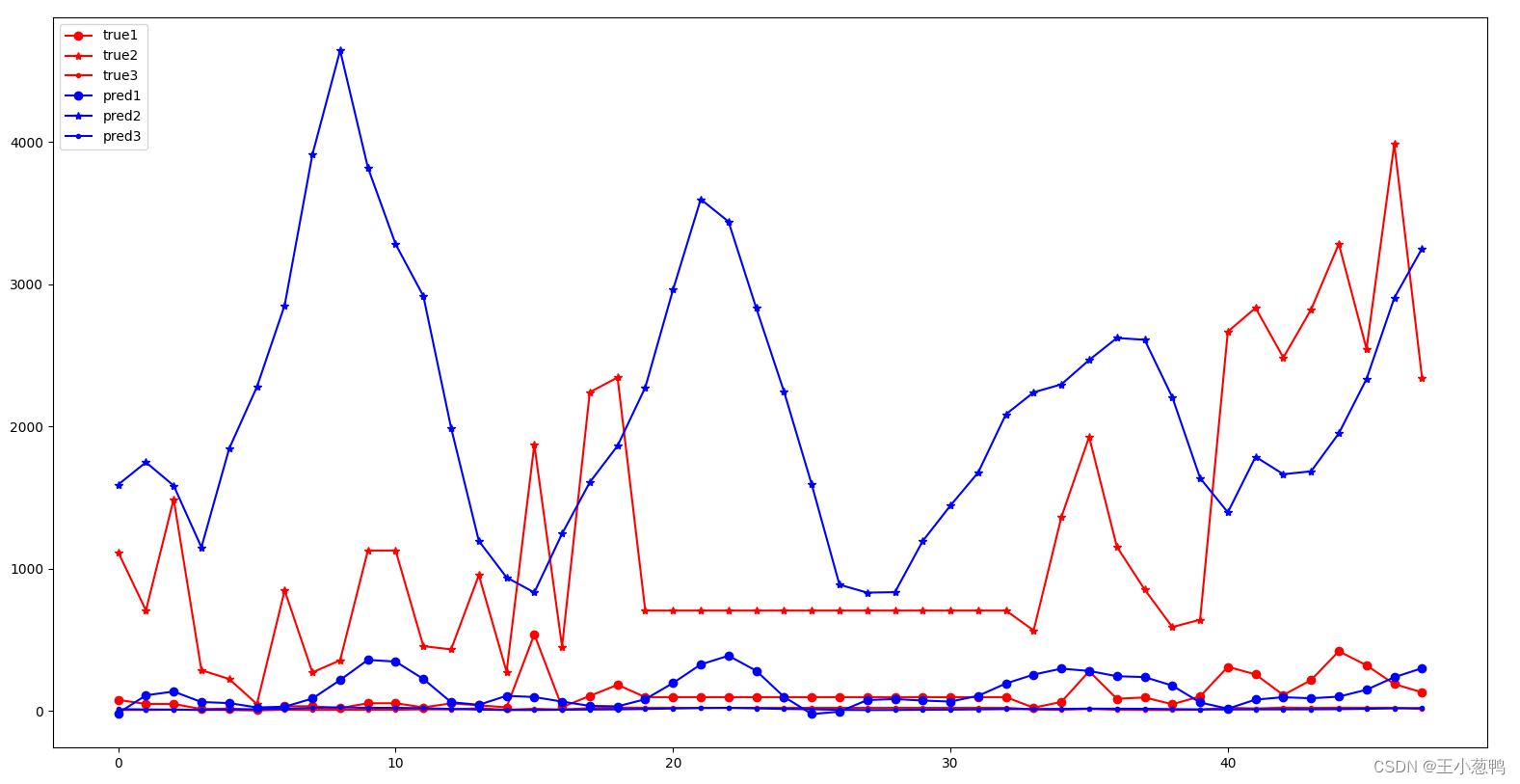
3.4 结果可视化

loss图像

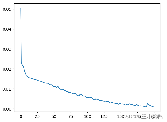
最后3个变量的预测结果，看出能预测大体趋势，但是数据集质量不高，导致最后的结果不好，模型也需要继续优化。

完整代码和数据集，关注公众号：AI学习部 ，发送“时间序列”关键词获取，或联系Q 596520206。