


神经网络核心任务:找出最佳W
一、梯度下降法优化权重数组W
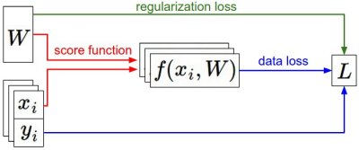
在神经网络的训练中主要是寻找针对损失函数(loss)最小的参数值W的值(有时候称为权重数组weight vector)。关于权重数组的优化有很多种方式。
1)尝试
尝试1:无脑的Random search
思路就是不间断地给权重数组赋随机值,取最好的结果,以下代码举例,最优权重数组为bestW。通过该方法训练得到的W测试后准确率只有12%。
# assume X_train is the data where each column is an example (e.g. 3073 x 50,000)
# assume Y_train are the labels (e.g. 1D array of 50,000)
# assume the function L evaluates the loss function

bestloss = float("inf") # Python assigns the highest possible float value
for num in xrange(1000):
  W = np.random.randn(10, 3073) * 0.0001 # generate random parameters
  loss = L(X_train, Y_train, W) # get the loss over the entire training set
  if loss < bestloss: # keep track of the best solution
    bestloss = loss
    bestW = W
  print(in attempt %d the loss was %f, best %f' % (num, loss, bestloss))
尝试2:Random Local Search
先给一个随机的W,在Local Random下取随机值,得到最优的结果。通过该方法训练得到的W测试后准确率也只有21%。
W = np.random.randn(10, 3073) * 0.001 # generate random starting W
bestloss = float("inf")
for i in xrange(1000):
  step_size = 0.0001
  Wtry = W + np.random.randn(10, 3073) * step_size
  loss = L(Xtr_cols, Ytr, Wtry)
  if loss < bestloss:
    W = Wtry
    bestloss = loss
  print(iter %d loss is %f' % (i, bestloss))
2)梯度下降
在前两个方法中,我们都根据损失函数(loss)这一个目标,在权重空间中随意寻找,以提高权重数组对于预测的准确性。结果显示,随机的搜索对于准确方向的把控并没有起到作用。为了损失函数趋于0这一个总目标,我们可以用数学的方法去计算权重改变的方向,这一个方向就是梯度。
二、Learning Rate的选择
函数梯度告诉了我们函数变化最迅速的方向,但是我们要在这一方向上走多少需要自己把控,走的步长称为step size(有时候也叫学习率learning rate)。

正确的步长选择也是神经网络训练的重要参数设置组成部分,如果选择的步长很小,那么我们有时候花费了很长时间却取得了很小的进步;反之,如果选择步长很大,可能产生更大的loss,称之为"overstep"。合适的学习率是在能保证收敛的情况下尽快收敛,具体可参考如下。
Effect of step size. The gradient tells us the direction in which the function has the steepest rate of increase, but it does not tell us how far along this direction we should step. As we will see later in the course, choosing the step size (also called the learning rate) will become one of the most important (and most headache-inducing) hyperparameter settings in training a neural network. In our blindfolded hill-descent analogy, we feel the hill below our feet sloping in some direction, but the step length we should take is uncertain. If we shuffle our feet carefully we can expect to make consistent but very small progress (this corresponds to having a small step size). Conversely, we can choose to make a large, confident step in an attempt to descend faster, but this may not pay off. As you can see in the code example above, at some point taking a bigger step gives a higher loss as we “overstep”.
三、Mini-batch gradient descent(MBGD)
有时候训练参数有上百万个数据集,显然只是为了完成一些参数的更新,将损失函数在整个数据集上训练显然是计算浪费的。(it seems wasteful to compute the full loss function over the entire training set in order to perform only a single parameter update)解决这一个困难非常通用的方法就是在所有的训练数据中提取一组batch来计算梯度。举个例子,在如今的卷积神经网络中,通常典型的从训练数据集百万个样本中,取一个包含256个样本作为batch。
我们其实在做Gradient descent的时候,我们并不会真的去minimize total loss(即不会用BGD),而是使用mini-batch。
我们是怎么做的呢?我们会把training data分成一个一个的batch。比如说有1万张图片,每次随机选100张进来作为一个batch,一共有100个batch。每个batch要随机的分,如果batch没有随机的分,比如说某一个batch里面统统都是1,另一个batch里面统统都是数字2,这样会对performance会有不小的影响。Keras会帮你随机的放,不需要自己写。
# Vanilla Minibatch Gradient Descent

while True:
  data_batch = sample_training_data(data, 256) # sample 256 examples
  weights_grad = evaluate_gradient(loss_fun, data_batch, weights)
  weights += - step_size * weights_grad # perform parameter update
这一个方法可行的原因是训练数据样本都是想关联的。To see this, consider the extreme case where all 1.2 million images in ILSVRC are in fact made up of exact duplicates of only 1000 unique images (one for each class, or in other words 1200 identical copies of each image). Then it is clear that the gradients we would compute for all 1200 identical copies would all be the same, and when we average the data loss over all 1.2 million images we would get the exact same loss as if we only evaluated on a small subset of 1000. In practice of course, the dataset would not contain duplicate images, the gradient from a mini-batch is a good approximation of the gradient of the full objective. Therefore, much faster convergence can be achieved in practice by evaluating the mini-batch gradients to perform more frequent parameter updates.
四、Stochastic Gradient Descent (SGD)
The extreme case of this is a setting where the mini-batch contains only a single example. This process is called Stochastic Gradient Descent (SGD) (or also sometimes on-line gradient descent). This is relatively less common to see because in practice due to vectorized code optimizations it can be computationally much more efficient to evaluate the gradient for 100 examples, than the gradient for one example 100 times. Even though SGD technically refers to using a single example at a time to evaluate the gradient, you will hear people use the term SGD even when referring to mini-batch gradient descent (i.e. mentions of MGD for “Minibatch Gradient Descent”, or BGD for “Batch gradient descent” are rare to see), where it is usually assumed that mini-batches are used. The size of the mini-batch is a hyperparameter but it is not very common to cross-validate it. It is usually based on memory constraints (if any), or set to some value, e.g. 32, 64 or 128. We use powers of 2 in practice because many vectorized operation implementations work faster when their inputs are sized in powers of 2.
【1】优化梯度下降总纲:https://ruder.io/optimizing-gradient-descent/
【2】部分内容摘自:https://cs231n.github.io/optimization-1/
【3】batch:https://blog.csdn.net/pengchengliu/article/details/89215659


 13万+
13万+


 被折叠的 条评论
为什么被折叠?
被折叠的 条评论
为什么被折叠?
 到【灌水乐园】发言


