


文章目录
Autogluon是一个开源的自动机器学习框架,由AWS(亚马逊网络服务)开发和维护。它旨在简化机器学习的流程,使得即使对机器学习不熟悉的用户也能够轻松地构建高性能的机器学习模型。
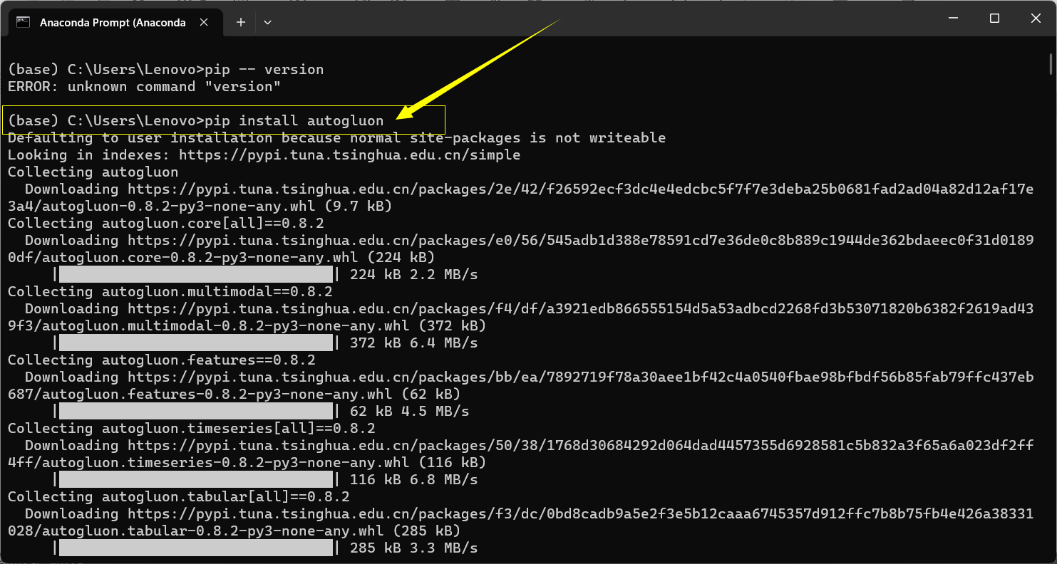
一、安装
打开Anaconda Prompt 输入 pip install autogluon
二、示例一 AutoGluon预测目标数据
在这个示例中,Autogluon被用于自动化地进行表格数据的特征工程、模型选择和超参数调优。具体来说,Autogluon可以自动处理表格数据的缺失值、类别特征的编码、特征选择等预处理步骤。然后,Autogluon会自动选择适合数据集的机器学习模型,并进行模型的训练和调优。
1、导入数据
使用 AutoGluon 根据表格数据集中的其他列预测目标列的值。
from autogluon.tabular import TabularDataset, TabularPredictor
在本教程中,我们将使用 《自然》第 7887 期封面故事 中的数据集:数学定理的 AI 引导直觉。目标是根据结的属性预测结的特征。我们从原始数据中抽取了 10K 训练和 5K 测试示例。采样数据集使本教程运行速度很快,但如果需要,AutoGluon 可以处理完整的数据集。
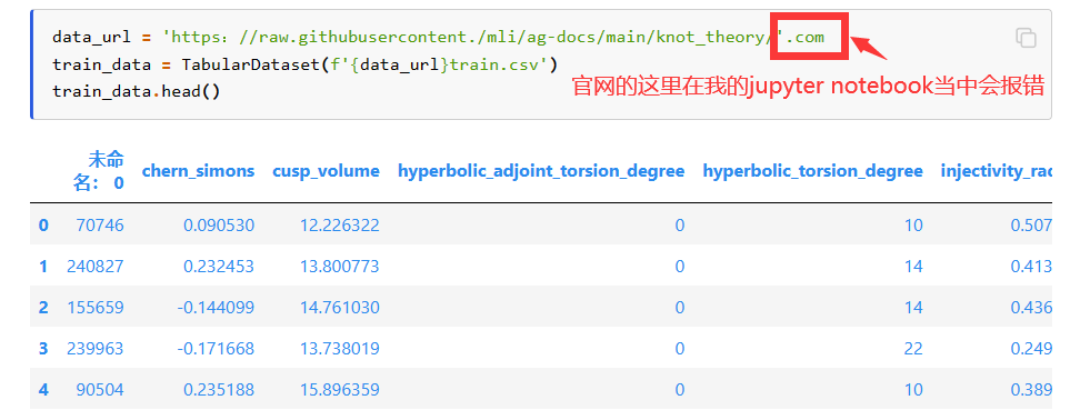
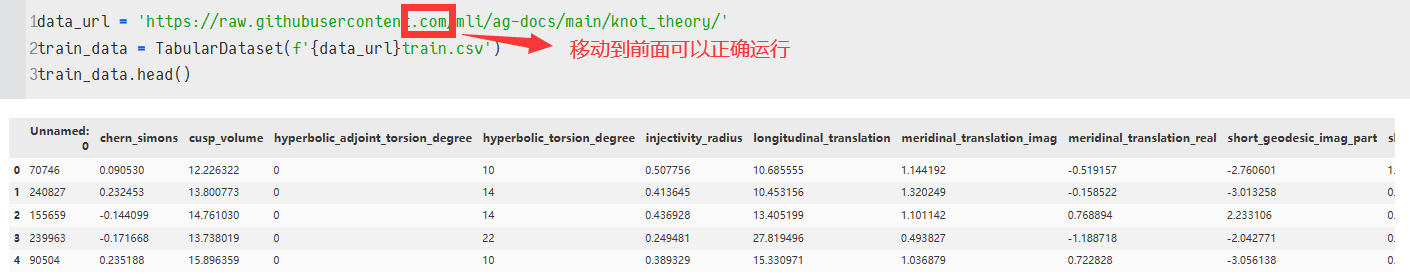
我们直接从 URL 加载此数据集。AutoGluon是pandas DataFrame的一个子类,所以任何方法都可以使用。
data_url = 'https://raw.githubusercontent.com/mli/ag-docs/main/knot_theory/'
train_data = TabularDataset(f'{data_url}train.csv')
train_data.head()
我们的目标存储在“签名”列中,该列有 18 个唯一整数。即使 pandas 没有正确识别此数据类型为分类,AutoGluon 也会解决此问题。
label = 'signature'
train_data[label].describe()
count    10000.000000
mean        -0.022000
std          3.025166   # 标准差
min        -12.000000
25%         -2.000000
50%          0.000000
75%          2.000000
max         12.000000
Name: signature, dtype: float64
2、训练
AutoGluon将识别这是一个多类分类任务,执行自动特征工程,训练多个模型,然后集成模型以创建最终预测器。
predictor = TabularPredictor(label=label).fit(train_data)
模型拟合应该需要几分钟或更短的时间,具体取决于您的 CPU。可以通过指定参数来加快训练速度。例如,将在 60 秒后停止训练。较高的时间限制通常会导致更好的预测性能,而过低的时间限制将阻止 AutoGluon 训练和组装一组合理的模型。
我跑出来的结果,感觉还是CPU弱了:
Fitting 13 L1 models ...
Fitting model: KNeighborsUnif ...
	0.2232	 = Validation score   (accuracy)
	4.97s	 = Training   runtime
	0.04s	 = Validation runtime
Fitting model: KNeighborsDist ...
	0.2132	 = Validation score   (accuracy)
	0.13s	 = Training   runtime
	0.02s	 = Validation runtime
Fitting model: NeuralNetFastAI ...
	0.9469	 = Validation score   (accuracy)
	17.21s	 = Training   runtime
	0.04s	 = Validation runtime
Fitting model: LightGBMXT ...
	0.9459	 = Validation score   (accuracy)
	7.29s	 = Training   runtime
	0.06s	 = Validation runtime
Fitting model: LightGBM ...
	0.956	 = Validation score   (accuracy)
	5.09s	 = Training   runtime
	0.03s	 = Validation runtime
Fitting model: RandomForestGini ...
	0.9449	 = Validation score   (accuracy)
	1.99s	 = Training   runtime
	0.12s	 = Validation runtime
Fitting model: RandomForestEntr ...
	0.9499	 = Validation score   (accuracy)
	2.36s	 = Training   runtime
	0.09s	 = Validation runtime
Fitting model: CatBoost ...
	0.956	 = Validation score   (accuracy)
	59.54s	 = Training   runtime
	0.01s	 = Validation runtime
Fitting model: ExtraTreesGini ...
	Warning: Reducing model 'n_estimators' from 300 -> 199 due to low memory. Expected memory usage reduced from 22.54% -> 15.0% of available memory...
	0.9479	 = Validation score   (accuracy)
	0.89s	 = Training   runtime
	0.06s	 = Validation runtime
Fitting model: ExtraTreesEntr ...
	Warning: Reducing model 'n_estimators' from 300 -> 184 due to low memory. Expected memory usage reduced from 24.35% -> 15.0% of available memory...
	0.9369	 = Validation score   (accuracy)
	1.06s	 = Training   runtime
	0.07s	 = Validation runtime
Fitting model: XGBoost ...
	0.957	 = Validation score   (accuracy)
	9.9s	 = Training   runtime
	0.06s	 = Validation runtime
Fitting model: NeuralNetTorch ...
	0.9409	 = Validation score   (accuracy)
	67.47s	 = Training   runtime
	0.01s	 = Validation runtime
Fitting model: LightGBMLarge ...
	0.9499	 = Validation score   (accuracy)
	11.85s	 = Training   runtime
	0.22s	 = Validation runtime
Fitting model: WeightedEnsemble_L2 ...
	0.965	 = Validation score   (accuracy)
	0.69s	 = Training   runtime
	0.0s	 = Validation runtime
AutoGluon training complete, total runtime = 194.08s ... Best model: "WeightedEnsemble_L2"
TabularPredictor saved. To load, use: predictor = TabularPredictor.load("AutogluonModels\ag-20230719_064926\")
3、预测
一旦我们有了适合训练数据集的预测器,我们就可以加载一组单独的数据来用于预测和评估。
test_data = TabularDataset(f'{data_url}test.csv')

y_pred = predictor.predict(test_data.drop(columns=[label]))
y_pred.head()
0   -4
1   -2
2    0
3    4
4    2
Name: signature, dtype: int64
4、评估
我们可以使用该函数在测试数据集上评估预测因子,该函数衡量我们的预测器在未用于拟合模型的数据上的表现。
predictor.evaluate(test_data, silent=True)
AutoGluon还提供了该功能,它允许我们在测试数据上评估每个训练模型的性能。
predictor.leaderboard(test_data, silent=True)

5、小结
AutoGluon 无需特征工程或模型超参数调优,简化了模型训练过程。
三、示例二 AutoGluon多模态预测(Multimodal Prediction)
在本示例中,Autogluon被用于训练一个模型,该模型可以根据输入的文本和图像来预测宠物的年龄。
在这个示例中,使用了一个包含宠物的图像和它们的描述文本的数据集。Autogluon通过将文本和图像作为输入,自动学习如何将它们结合起来进行预测。
即使用了深度学习模型来处理图像数据,并将文本数据转化为特征向量。然后,Autogluon将这些特征向量输入到一个集成模型中,以进行最终的预测。
其中,宠物的图片是通过使用深度学习模型进行处理的。具体来说,使用了一个预训练的图像分类模型(ResNet-50)来提取图像的特征。这些特征被用作输入,与文本特征一起输入到集成模型中进行预测。
1、导入数据
在本示例中,我们使用 PetFinder 数据集的简化和子采样版本。目标是根据宠物的收养概况预测宠物的收养率。在这个简化版本中,宠物收养速度(AdoptionSpeed)分为两类:0(慢)和1(快)。我们首先下载一个包含 petfinder 数据集的 zip 文件,并在当前工作目录中解压缩它们。
from autogluon.core.utils.loaders import load_zip

download_dir = './ag_multimodal_tutorial'
zip_file = 'https://automl-mm-bench.s3.amazonaws.com/petfinder_for_tutorial.zip'

load_zip.unzip(zip_file, unzip_dir=download_dir)
接下来,我们使用 pandas 将数据集的 CSV 文件读入 ,注意我们有兴趣学习预测的列是“收养速度”(AdoptionSpeed)。
import pandas as pd

dataset_path = f'{download_dir}/petfinder_for_tutorial'

train_data = pd.read_csv(f'{dataset_path}/train.csv', index_col=0)
test_data = pd.read_csv(f'{dataset_path}/test.csv', index_col=0)

label_col = 'AdoptionSpeed'
PetFinder 数据集附带一个图像目录,数据中的某些记录具有多个与之关联的图像。AutoGluon 的多模式数据帧格式要求图像列包含一个字符串,其值是单个图像文件的路径。对于此示例,我们将图像功能列限制为仅第一个图像,并且需要执行一些路径操作才能为当前目录结构正确设置所有内容。
image_col = 'Images' # 定义一个变量image_col,用于表示图像路径所在的列名。

train_data[image_col] = train_data[image_col].apply(lambda ele: ele.split(';')[0])
# 对训练数据集中的image_col列的每个元素进行操作。使用apply函数和匿名函数,将每个元素按照分号进行分割,并将分割后的第一个元素赋值给原来的位置。

test_data[image_col] = test_data[image_col].apply(lambda ele: ele.split(';')[0])
# 对测试数据集中的image_col列的每个元素进行相同的操作,将分割后的第一个元素赋值给原来的位置。

def path_expander(path, base_folder):
# 定义了一个名为path_expander的函数,该函数接受两个参数:path表示图像路径,base_folder表示基础文件夹路径。
    path_l = path.split(';') # 将传入的图像路径按照分号进行分割,得到一个路径列表。
    return ';'.join([os.path.abspath(os.path.join(base_folder, path)) for path in path_l])
# 对路径列表中的每个路径进行处理,使用os.path.join函数将基础文件夹路径和每个路径进行拼接,并使用os.path.abspath函数获取绝对路径。然后,使用';'.join函数将处理后的路径列表重新拼接成一个字符串,以分号作为分隔符。

train_data[image_col] = train_data[image_col].apply(lambda ele: path_expander(ele, base_folder=dataset_path))
test_data[image_col] = test_data[image_col].apply(lambda ele: path_expander(ele, base_folder=dataset_path))
上面这段代码的目的是对数据集中的图像路径进行处理。首先,通过分割操作去除了路径中的附加信息,只保留了第一个元素。然后,使用path_expander函数将路径拼接为绝对路径,并将处理后的路径赋值给原来的位置。这样可以确保图像路径的正确性和一致性。
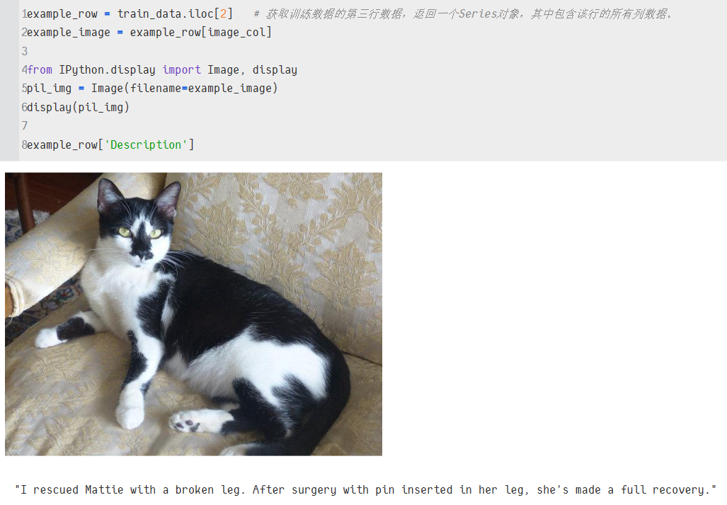
每种动物的领养资料包括图片、文本描述和各种表格特征,如年龄、品种、名称、颜色等。让我们看一下示例数据行的图片和说明。
example_row = train_data.iloc[2]
 # 获取训练数据的第三行数据,返回一个Series对象,其中包含该行的所有列数据。(因为iloc是从0开始的)
example_image = example_row[image_col]

from IPython.display import Image, display
pil_img = Image(filename=example_image)
display(pil_img)

example_row['Description']
2、训练
设置训练时间为120秒。(更多的训练时间将导致更好的预测性能,但我们可以在短时间内获得令人惊讶的良好性能。)
from autogluon.multimodal import MultiModalPredictor

predictor = MultiModalPredictor(label=label_col).fit(
    train_data=train_data,
    time_limit=120
)
在后台自动推断问题类型(分类或回归),检测特征模态,从多模态模型池中选择模型,并训练所选模型。如果使用多个主干,MultiModalPredictor会在它们之上附加一个后期融合模型(MLP或变压器)。
3、预测
拟合模型后,我们希望使用它来预测 witheld 测试数据集中的标签。
predictions = predictor.predict(test_data.drop(columns=label_col))
predictions[:5]
0表示收养速度慢,1表示收养速度快。
8     0
70    1
82    1
28    0
63    1
Name: AdoptionSpeed, dtype: int64
对于分类任务,我们可以很容易地获得每个输出类的预测概率。
probs = predictor.predict_proba(test_data.drop(columns=label_col))
probs[:5]
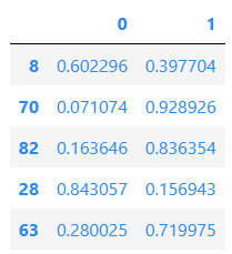
4、评估
最后,我们可以评估其他性能指标(在本例中为roc_auc)的 witheld 测试数据集上的预测因子。
scores = predictor.evaluate(test_data, metrics=["roc_auc"])
scores
{'roc_auc': 0.914}
四、示例三 多模态自动对文本与时间数据进行处理
import pandas as pd
from sklearn.model_selection import train_test_split
from autogluon.tabular import TabularDataset, TabularPredictor
label = "label"
X=dfA
y = dfA[['label']]
#划分数据集并使用autogluon自动训练,  可根据需要指定预测方式problem_type=‘regression’: 回归问题;‘classfication’: 分类问题
train_x,test_x,train_y,test_y=train_test_split(X,y,test_size=0.05,random_state=0)
from autogluon.tabular import FeatureMetadata
feature_metadata = FeatureMetadata.from_df(train_x)

print(feature_metadata)

feature_metadata = feature_metadata.add_special_types({'thedate': ['datetime_as_object'],'summary': ['text']})
print(feature_metadata)

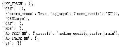
from autogluon.tabular.configs.hyperparameter_configs import get_hyperparameter_config
# 多模态训练模式
hyperparameters = get_hyperparameter_config('multimodal')
hyperparameters
from autogluon.tabular import TabularPredictor
predictor = TabularPredictor(label=label,path="REmodel").fit(
    train_data=train_x,
    hyperparameters=hyperparameters,
    feature_metadata=feature_metadata,
    presets = 'good_quality',
    time_limit=3*3600,
    ag_args_fit={'num_gpus': 1})
注:ag_args_fit={'num_gpus': 1} 这个参数我运行的时候会报错,在实际跑的过程当中直接删除就行了。
leaderboard = predictor.leaderboard(test_x) # 生成预测模型的排行榜
注:autogluon可以自动识别预测的数据是回归问题还是分类问题。
五、示例四 AutoGluon进行时间序列预测
通过一个简单的调用,AutoGluon可以训练和调整fit()
- 简单的预测模型(例如,ARIMA,ETS,Theta),
- 强大的深度学习模型(例如,DeepAR,时间融合变压器),
- 基于树的模型(例如,LightGBM),
- 结合其他模型预测的融合
- 为单变量时间序列数据生成多步提前概率预测。
本教程演示如何快速开始使用 AutoGluon 为 M4 预测竞赛数据集生成每小时预测。
1、导入数据
import pandas as pd
from autogluon.timeseries import TimeSeriesDataFrame, TimeSeriesPredictor
-
TimeSeriesDataFrame存储由多个时间序列组成的数据集。 -
TimeSeriesPredictor负责拟合、调整和选择最佳预测模型,以及生成新的预测。
df = pd.read_csv("https://autogluon.s3.amazonaws.com/datasets/timeseries/m4_hourly_subset/train.csv")
df.head()
官网直接读取慢。。网不好。。
AutoGluon 需要长格式的时间序列数据。 数据框的每一行都包含由表示单个时间序列的单个观测值(时间步长)
-
时间序列的唯一ID: int 或 str"item_id"
-
观测值的时间戳:"timestamp"pandas.Timestamp
-
时间序列的数值:(“target”)
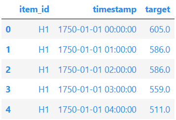
原始数据集应始终遵循此格式,其中唯一 ID、时间戳和目标值至少有三列,但这些列的名称可以是任意的。 但重要的是,在构造 AutoGluon 使用的列时,我们要提供列的名称。 如果数据与预期格式不匹配,AutoGluon 将引发异常。
train_data = TimeSeriesDataFrame.from_data_frame(
    df,
    id_column="item_id",
    timestamp_column="timestamp"
)
train_data.head()

2、训练
为了预测时间序列的未来值,我们需要创建一个对象。
预测时间序列中的模型将多步推向未来。 我们根据任务选择这些步骤的数量——预测长度(也称为预测范围)。 例如,我们的数据集包含按小时频率测量的时间序列,因此我们设置为训练预测未来 48 小时的模型。
我们指示 AutoGluon 将训练好的模型保存在文件夹中。 我们还指定 AutoGluon 应根据平均绝对标度误差 (MASE) 对模型进行排名,并且我们要预测的数据存储在 ../autogluon-m4-hourly"target"TimeSeriesDataFrame
predictor = TimeSeriesPredictor(
    prediction_length=48, # 预测未来 48 小时的模型
    path="autogluon-m4-hourly",
    target="target", # 要预测的数据存储在target
    eval_metric="MASE",
)

predictor.fit(
    train_data,
    presets="medium_quality",
    time_limit=600,
)
================ TimeSeriesPredictor ================
TimeSeriesPredictor.fit() called
Setting presets to: medium_quality
Fitting with arguments:
{'enable_ensemble': True,
 'evaluation_metric': 'MASE',
 'excluded_model_types': None,
 'hyperparameter_tune_kwargs': None,
 'hyperparameters': 'medium_quality',
 'num_val_windows': 1,
 'prediction_length': 48,
 'random_seed': None,
 'target': 'target',
 'time_limit': 600,
 'verbosity': 2}
Provided training data set with 148060 rows, 200 items (item = single time series). Average time series length is 740.3. Data frequency is 'H'.
=====================================================
AutoGluon will save models to autogluon-m4-hourly/
AutoGluon will gauge predictive performance using evaluation metric: 'MASE'
	This metric's sign has been flipped to adhere to being 'higher is better'. The reported score can be multiplied by -1 to get the metric value.

Provided dataset contains following columns:
	target:           'target'

Starting training. Start time is 2023-06-30 20:53:28
Models that will be trained: ['Naive', 'SeasonalNaive', 'Theta', 'AutoETS', 'RecursiveTabular', 'DeepAR']
Training timeseries model Naive. Training for up to 599.67s of the 599.67s of remaining time.
	-6.6629       = Validation score (-MASE)
	0.12    s     = Training runtime
	4.23    s     = Validation (prediction) runtime
Training timeseries model SeasonalNaive. Training for up to 595.31s of the 595.31s of remaining time.
	-1.2169       = Validation score (-MASE)
	0.12    s     = Training runtime
	0.22    s     = Validation (prediction) runtime
Training timeseries model Theta. Training for up to 594.96s of the 594.96s of remaining time.
	-2.1425       = Validation score (-MASE)
	0.11    s     = Training runtime
	28.11   s     = Validation (prediction) runtime
Training timeseries model AutoETS. Training for up to 566.74s of the 566.74s of remaining time.
	-1.9399       = Validation score (-MASE)
	0.11    s     = Training runtime
	102.47  s     = Validation (prediction) runtime
Training timeseries model RecursiveTabular. Training for up to 464.15s of the 464.15s of remaining time.
	-0.8988       = Validation score (-MASE)
	14.11   s     = Training runtime
	2.43    s     = Validation (prediction) runtime
Training timeseries model DeepAR. Training for up to 447.60s of the 447.60s of remaining time.
	-1.8466       = Validation score (-MASE)
	93.08   s     = Training runtime
	2.04    s     = Validation (prediction) runtime
Fitting simple weighted ensemble.
	-0.8824       = Validation score (-MASE)
	5.73    s     = Training runtime
	107.15  s     = Validation (prediction) runtime
Training complete. Models trained: ['Naive', 'SeasonalNaive', 'Theta', 'AutoETS', 'RecursiveTabular', 'DeepAR', 'WeightedEnsemble']
Total runtime: 253.34 s
Best model: WeightedEnsemble
Best model score: -0.8824
3、预测
现在,我们可以使用拟合来预测未来的时间序列值。 默认情况下,AutoGluon 将使用在内部验证集中得分最高的模型进行预测。 预测始终包括对下一个时间步长的预测,从 中每个时间序列的末尾开始。
predictions = predictor.predict(train_data)
predictions.head()
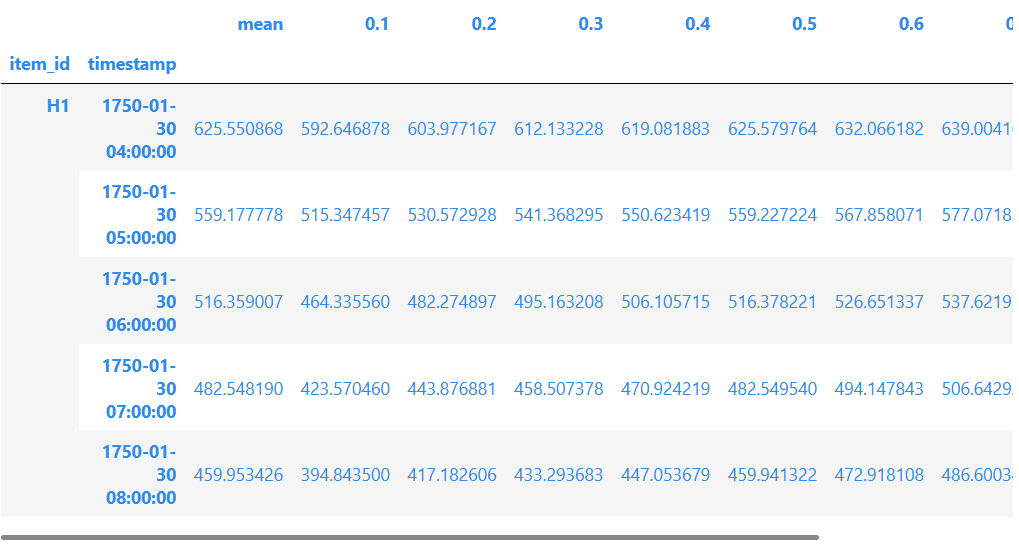
AutoGluon 生成概率预测:除了预测未来时间序列的平均值(期望值)外,模型还提供预测分布的分位数。 分位数预测让我们了解可能结果的范围。
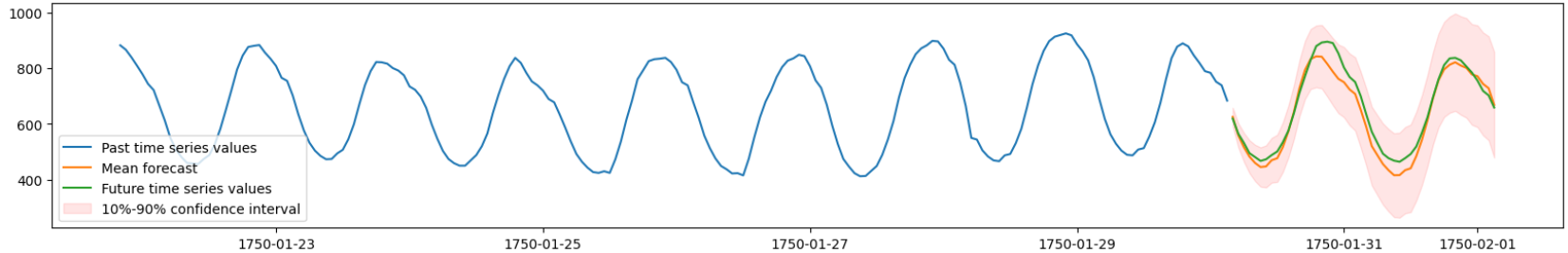
现在,我们将可视化数据集中某个时间序列的预测和实际观测值。 我们绘制平均预测以及 10% 和 90% 分位数以显示潜在结果的范围。
import matplotlib.pyplot as plt

# TimeSeriesDataFrame can also be loaded directly from a file
test_data = TimeSeriesDataFrame.from_path("https://autogluon.s3.amazonaws.com/datasets/timeseries/m4_hourly_subset/test.csv")

plt.figure(figsize=(20, 3))

item_id = "H1"
y_past = train_data.loc[item_id]["target"]
y_pred = predictions.loc[item_id]
y_test = test_data.loc[item_id]["target"][-48:]

plt.plot(y_past[-200:], label="Past time series values")
plt.plot(y_pred["mean"], label="Mean forecast")
plt.plot(y_test, label="Future time series values")

plt.fill_between(
    y_pred.index, y_pred["0.1"], y_pred["0.9"], color="red", alpha=0.1, label=f"10%-90% confidence interval"
)
plt.legend();
4、评估
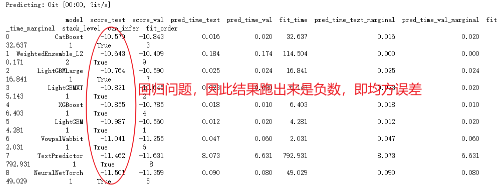
我们可以查看 AutoGluon 通过该方法训练的每个模型的性能。 我们为排行榜函数提供测试数据集,以查看拟合模型在看不见的测试数据上的表现如何。 排行榜还包括在内部验证数据集上计算的验证分数。
在 AutoGluon 排行榜中,分数越高,预测性能越好。
# The test score is computed using the last
# prediction_length=48 timesteps of each time series in test_data
predictor.leaderboard(test_data, silent=True)


 4471
4471


 被折叠的 条评论
为什么被折叠?
被折叠的 条评论
为什么被折叠?
 到【灌水乐园】发言


