tensorflow多元线性回归

多元线性回归，数据集为boston房价与周边环境等因素，以下为代码

#2021.10.13 HIT ATCI LZH
#多元线性回归，数据集为boston房价与周边环境等因素，参照网上的例子
import tensorflow as tf
from tensorflow.python.ops import init_ops
from tensorflow.python.training import optimizer  
import numpy as np
import matplotlib.pyplot as plt
#加载boston房价数据集
boston = tf.contrib.learn.datasets.load_dataset('boston')
X_train, Y_train = boston.data, boston.target
#对数据集的格式进行解析
print('数据加载成功！')
print('boston.type is',type(boston))
print('X_train.type =', type(X_train))
print('X_train.ndim =',X_train.ndim)
print('X_train.shape =',X_train.shape)
print('X_train.dtype =',X_train.dtype)
print('X_train 的行数 m = {0}, 列数 n = {1}'.format(X_train.shape[0],X_train.shape[1]))
print('Y_train.type =', type(Y_train))
print('Y_train.ndim =',Y_train.ndim)
print('Y_train.shape =',Y_train.shape)
print('Y_train 的行数 m = {0}, 列数 n = None'.format(Y_train.shape[0]))
print('Y_train.dtype =',Y_train.dtype)
#因为各特征的数据范围不同，需要归一化特征数据
#定义归一化函数
def normalize(X):
    mean = np.mean(X) #均值
    std = np.std(X)  #默认计算每一列的标准差
    X = (X - mean)/std
    return X
#定义一个额外的固定输入权重与偏置结合起来，该技巧可以有效的简化编程
def append_bias_reshape(features, labels):
    m = features.shape[0] #行数
    n = features.shape[1] #列数
    x = np.reshape(np.c_[np.ones(m), features],[m, n+1])
    y = np.reshape(labels, [m, 1]) #将lables由向量变为矩阵
    return x,y
X_train = normalize(X_train) #对输入变量按列进行归一化
X_train, Y_train = append_bias_reshape(X_train, Y_train) #对X_train进行处理，增加一列全1向量，处理后只有矩阵相乘，可以省略掉偏置相加的过程
m = len(X_train) #训练集样本数量
n = X_train.shape[1] #number of features + biases
print(n)
#对归一化的效果进行查看

#为训练数据申明Tensorflow占位符
X = tf.placeholder(tf.float32,shape = [m , n], name='X') #每次训练全部导入数据，bitchsize就是全部数据集，因此shape = [m , n]
Y = tf.placeholder(tf.float32, name='Y')
#创建Tensorflow的权重和偏置且初始值设为0
w = tf.Variable(tf.random_normal([n, 1])) 
#由于定义了函数append_bias_reshape, 因此不需要b = tf.Variable(0.0) 
#b = tf.Variable(0.0)
#定义用于预测的线性回归模型
Y_hat = tf.matmul(X, w)
#定义损失函数
loss = tf.reduce_mean(tf.square(Y - Y_hat))#损失函数，均方误差
#选择梯度下降优化器,并设置学习率
optimizer = tf.train.GradientDescentOptimizer(learning_rate=0.01).minimize(loss) #学习率
#申明初始化操作符
init_op = tf.global_variables_initializer()
total = []#定义一个空列表
#启动计算图
with tf.Session() as sess:
    sess.run(init_op)#初始化变量
    for i in range(100):
        _, l = sess.run([optimizer, loss],feed_dict = {X:X_train, Y:Y_train})
        total.append(l)
        print('Epoch {0}: Loss {1}'.format(i, l))
    w_value = sess.run(w)
    #print(b_value)
    #print(w_value)
#绘制损失函数
plt.figure(num=1)
plt.title('loss')
plt.plot(total)
plt.show()

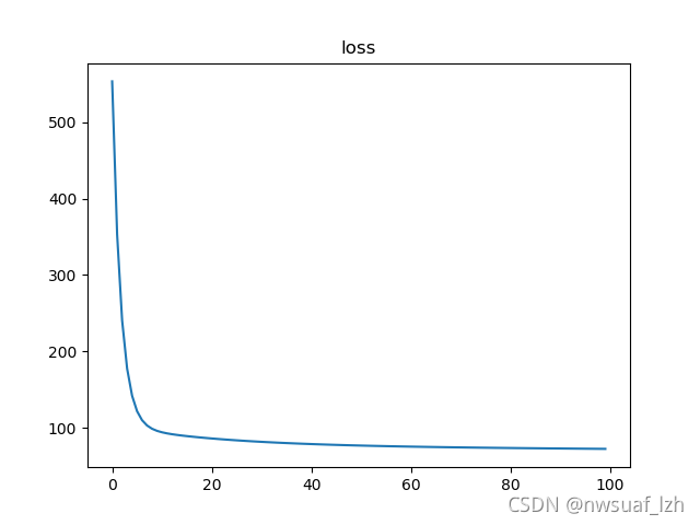
由上图我们可以发现，当Epoch大于20之后，loss的变化趋于平缓，这说明训练次数并非越多越好。 

2、还有一种编程思路是挨个儿把数据放到feed_dict中去 ，可以用zip函数进行遍历

#2021.10.13 HIT ATCI LZH
#多元线性回归，数据集为boston房价与周边环境等因素，参照网上的例子
import tensorflow as tf
from tensorflow.python.ops import init_ops
from tensorflow.python.training import optimizer  
import numpy as np
import matplotlib.pyplot as plt
#加载boston房价数据集
boston = tf.contrib.learn.datasets.load_dataset('boston')
X_train, Y_train = boston.data, boston.target
#对数据集的格式进行解析
print('数据加载成功！')
print('boston.type is',type(boston))
print('X_train.type =', type(X_train))
print('X_train.ndim =',X_train.ndim)
print('X_train.shape =',X_train.shape)
print('X_train.dtype =',X_train.dtype)
print('X_train 的行数 m = {0}, 列数 n = {1}'.format(X_train.shape[0],X_train.shape[1]))
print('Y_train.type =', type(Y_train))
print('Y_train.ndim =',Y_train.ndim)
print('Y_train.shape =',Y_train.shape)
print('Y_train 的行数 m = {0}, 列数 n = None'.format(Y_train.shape[0]))
print('Y_train.dtype =',Y_train.dtype)
#因为各特征的数据范围不同，需要归一化特征数据
#定义归一化函数
def normalize(X):
    mean = np.mean(X) #均值
    std = np.std(X)  #默认计算每一列的标准差
    X = (X - mean)/std
    return X
#定义一个额外的固定输入权重与偏置结合起来，该技巧可以有效的简化编程
def append_bias_reshape(features, labels):
    m = features.shape[0] #行数
    n = features.shape[1] #列数
    x = np.reshape(np.c_[np.ones(m), features],[m, n+1])
    y = np.reshape(labels, [m, 1]) #将lables由向量变为矩阵
    return x,y
X_train = normalize(X_train) #对输入变量按列进行归一化
X_train, Y_train = append_bias_reshape(X_train, Y_train) #对X_train进行处理，增加一列全1向量，处理后只有矩阵相乘，可以省略掉偏置相加的过程
m = len(X_train) #训练集样本数量
n = X_train.shape[1] #number of features + biases
print(n)
#对归一化的效果进行查看

#为训练数据申明Tensorflow占位符
X = tf.placeholder(tf.float32,shape = [None , n], name='X') #每次训练
Y = tf.placeholder(tf.float32, name='Y')
#创建Tensorflow的权重和偏置且初始值设为0
w = tf.Variable(tf.random_normal([n, 1])) 
#由于定义了函数append_bias_reshape, 因此不需要b = tf.Variable(0.0) 
#b = tf.Variable(0.0)
#定义用于预测的线性回归模型
Y_hat = tf.matmul(X, w)
#定义损失函数
loss = tf.reduce_mean(tf.square(Y - Y_hat))#损失函数，均方误差
#选择梯度下降优化器,并设置学习率
optimizer = tf.train.GradientDescentOptimizer(learning_rate=0.01).minimize(loss) #学习率
#申明初始化操作符
init_op = tf.global_variables_initializer()
total = []#定义一个空列表
#启动计算图
with tf.Session() as sess:
    sess.run(init_op)#初始化变量
    for i in range(100):
        epoch_loss = 0. #存储每导入一个数据的loss
        #_, l = sess.run([optimizer, loss],feed_dict = {X:X_train, Y:Y_train})
        for x,y in zip(X_train,Y_train):
            _, l = sess.run([optimizer, loss],feed_dict = {X:x.reshape([1,14]), Y:y}) #每feed进去一组数据便进行一次参数的训练
            epoch_loss += l
        total.append(epoch_loss/m)
        print('Epoch {0}: Loss {1}'.format(i, l))
    w_value = sess.run(w)
    #print(b_value)
    #print(w_value)
#绘制损失函数
plt.figure(num=1)
plt.title('loss')
plt.plot(total)
plt.show()

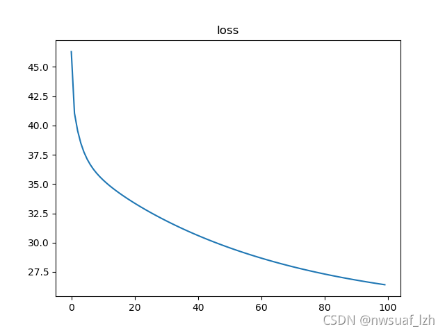
两种方法对比可以发现，第二种的loss在前几次的Epoch已经是非常小的，且每次Epoch都有明显的提升。