机器学习笔记2-Supervised learning

1.1 Probabilistic interpretation
why might the least-squares cost function J, be a reasonable choice?
Let us assume that the target variables and the inputs are related via the equation :

$${y^{(i)}}={{\theta}^{T}}{x^{(i)}}+{{\epsilon}^{(i)}}$$
${{\epsilon}^{(i)}}$ is an error term that captures either unmodeled effects or random noise.
Let us further assume that the ${{\epsilon}^{(i)}}$ are distributed IID (independently and identically distributed) .
$${{\epsilon}^{(i)}} ∼ N(0,σ2)$$
$$p({{\epsilon}^{(i)}})={\frac{1}{\sqrt{2{\pi}}{\sigma}}}exp{(-{\frac{({{\epsilon}^{(i)}})^2}{{\sigma}^2}})}$$
$$p({y^{(i)}}|{x^{(i)}};{{\theta}})={\frac{1}{\sqrt{2{\pi}}{\sigma}}}exp{(-{\frac{({y^{(i)}}-{{\theta}^{T}}{x^{(i)}})^2}{{\sigma}^2}})}$$
likelihood function：
$$L({\theta})=L({\theta};X,Y)=p(Y|X,{\theta})$$
$$={\prod_{i=1}^{m}}p({y^{(i)}}|{x^{(i)}};{{\theta}})$$
$$={\prod_{i=1}^{m}}{\frac{1}{\sqrt{2{\pi}}{\sigma}}}exp{(-{\frac{({y^{(i)}}-{{\theta}^{T}}{x^{(i)}})^2}{{\sigma}^2}})}$$
maximize the log likelihood
$$l({\theta})=logL({\theta})$$
$$=log{\prod_{i=1}^{m}}{\frac{1}{\sqrt{2{\pi}}{\sigma}}}exp{(-{\frac{({y^{(i)}}-{{\theta}^{T}}{x^{(i)}})^2}{{\sigma}^2}})}$$
$$={\sum_{i=1}^{m}}log{\frac{1}{\sqrt{2{\pi}}{\sigma}}}exp{(-{\frac{({y^{(i)}}-{{\theta}^{T}}{x^{(i)}})^2}{{\sigma}^2}})}$$
$$=mlog{\frac{1}{\sqrt{2{\pi}}{\sigma}}}-{\frac{1}{2}}{\frac{1}{{\sigma}^2}}{\sum_{i=1}^{m}}({y^{(i)}}-{{\theta}^{T}}{x^{(i)}})^2$$
Hence, maximizing $l({\theta})$ gives the same answer as minimizing ${\frac{1}{2}}{\sum_{i=1}^{m}}({y^{(i)}}-{{\theta}^{T}}{x^{(i)}})^2$
summarize: Under the previous probabilistic assumptions on the data, least-squares regression corresponds to finding the maximum likelihood estimate of θ.
1.2 Locally weighted linear regression
The leftmost figure below shows the result of fitting a $y = θ_0 + θ_1x$ to a dataset. We see that the data doesn’t really lie on straight line, and so the fit is not very good.

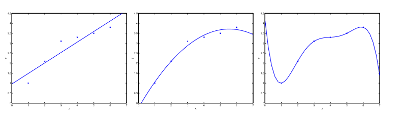
Instead, if we had added an extra feature $x^2$, and fit $y = θ_0 +θ_1x_1+θ_2x_2$, then we obtain a slightly better fit to the data. (See middle figure)
it might seem that the more features we add, the better. However, there is also a danger in adding too many features: The rightmost figure is the result of fitting a 5-th order polynomial $y={\sum_{j=0}^{5}{{\theta}_jx^j}}$ we’ll say the figure on the left shows an instance of underfitting—in which the data clearly shows structure not captured by the model—and the figure on the right is an example of overfitting.
As discussed previously, and as shown in the example above, the choice of features is important to ensuring good performance of a learning algorithm. (When we talk about model selection, we’ll also see algorithms for automatically choosing a good set of features.) In this section, let us talk briefly talk about the locally weighted linear regression (LWR) algorithm which, assuming there is sufficient training data, makes the choice of features less critical.
In the original linear regression algorithm, to make a prediction at a query point x .
1. Fit θ to minimize ${\sum_{i=1}^{m}}({y^{(i)}}-{{\theta}^{T}}{x^{(i)}})^2$
2. Output $θ^Tx$.
the locally weighted linear regression algorithm
1. Fit θ to minimize ${\sum_{i=1}^{m}}{\omega(i)}({y^{(i)}}-{{\theta}^{T}}{x^{(i)}})^2$
2. Output $θ^Tx$.
A fairly standard choice for the weights is：
$${\omega(i)}=exp{(-{\frac{({x^{(i)}}-x)^2}{2{\tau}^2}})}$$
if |x(i) − x| is small, then w(i) is close to 1; and if |x(i) − x| is large, then w(i) is small. Hence, θ is chosen giving a much higher “weight” to the (errors on) training examples close to the query point x.
The parameter τ controls how quickly the weight of a training example falls off with distance of its x(i) from the query point x; τ is called the bandwidth parameter.
Locally weighted linear regression is a non-parametric algorithm.The (unweighted) linear regression algorithm that we saw earlier is known as a parametric learning algorithm, because it has a fixed, finite number of parameters (the ${\theta}_i$ ), which are fit to the data. Once we’ve fit the ${\theta}_i$ and stored them away, we no longer need to keep the training data around to make future predictions. In contrast, to make predictions using locally weighted linear regression, we need to keep the entire training set around. The term “non-parametric” (roughly) refers to the fact that the amount of stuff we need to keep in order to represent the hypothesis h grows linearly with the size of the training set.