


ex1
load timeseriesAnalysis;
y_detrended1 = detrend(ydata1);
y_detrended2 = detrend(ydata2);
subplot(2,1,1);plot(x, ydata1,'-',x, ydata1-y_detrended1,'r');title('Detrended Signal 1');
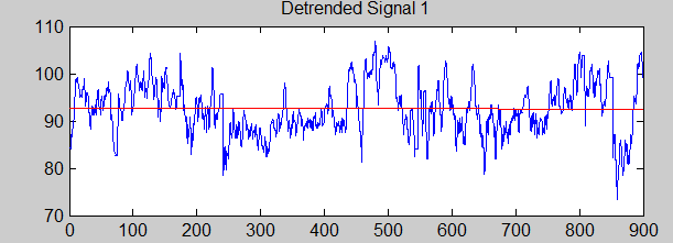
detrend 用法详见help.
ex2 如何使用scatter:
[attrib className] = xlsread('iris.xlsx');
%% basic scatter plot
figure('units','normalized','Position',[0.2359 0.3009 0.4094 0.6037]);
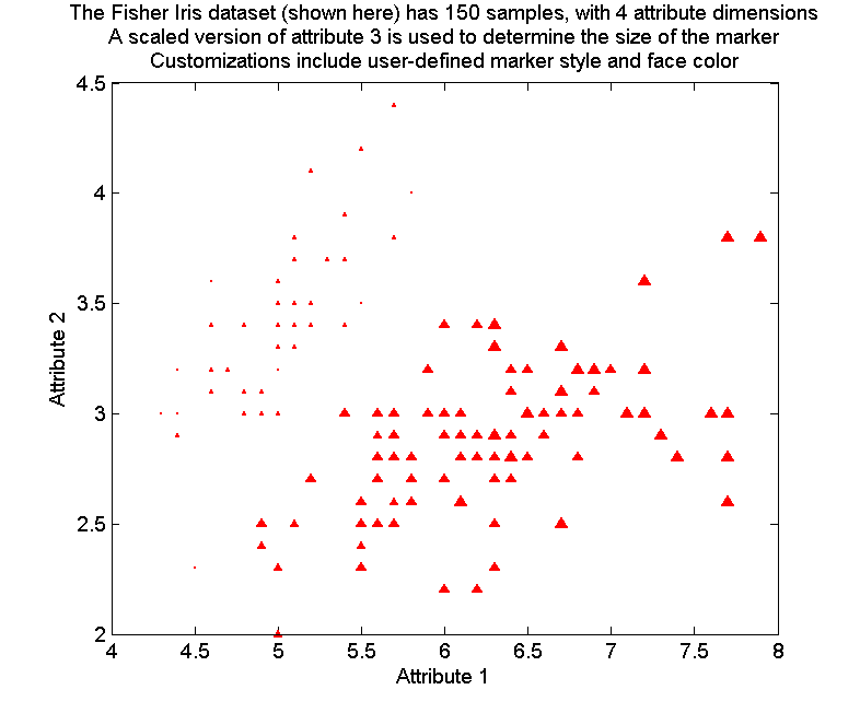
scatter(attrib(:,1),attrib(:,2),10*attrib(:,3),[1 0 0],'filled','Marker','^');
set(gca,'Fontsize',12);
title({'The Fisher Iris dataset (shown here) has 150 samples, with 4 attribute dimensions',...
'A scaled version of attribute 3 is used to determine the size of the marker',...
'Customizations include user-defined marker style and face color'});
xlabel('Attribute 1'); ylabel('Attribute 2');
box on;
set(gcf,'color',[1 1 1],'paperpositionmode','auto');
ex3:
%% plot matrix
% The output parameters have
% A matrix of handles to the objects created in H,
% A matrix of handles to the individual subaxes in AX,
% A handle to a big (invisible) axes that frames the subaxes in BigAx,
% A matrix of handles for the histogram plots in P. BigAx is left as the current axes so that a subsequent title, xlabel, or ylabel command is centered with respect to the matrix of axes.
figure('units','normalized','Position',[ 0.2359 0.3009 0.4094 0.6037]);
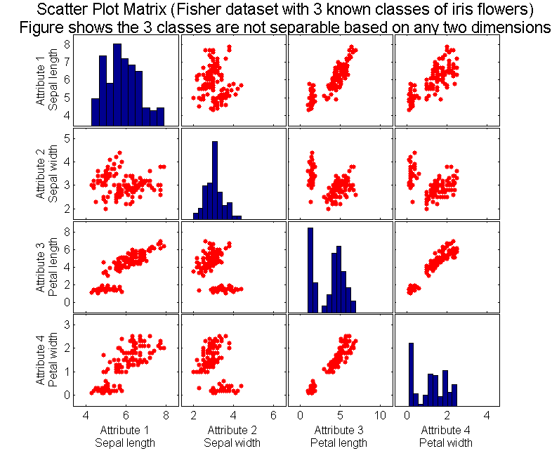
[H,AX,BigAx,P] = plotmatrix(attrib,'r.');
attribName = {[char(10) 'Sepal length'],[char(10) 'Sepal width'],[char(10) 'Petal length'],[char(10) 'Petal width']};
% add annotations
for i = 1:4
set(get(AX(i,1),'ylabel'),'string',['Attribute ' num2str(i) attribName{i}]);
set(get(AX(4,i),'xlabel'),'string',['Attribute ' num2str(i) attribName{i}]);
end
set(get(BigAx,'title'),'String',{'Scatter Plot Matrix (Fisher dataset with 3 known classes of iris flowers)', ...
'Figure shows the 3 classes are not separable based on any two dimensions'},'Fontsize',14);
set(gcf,'color',[1 1 1],'paperpositionmode','auto');
今天总结的很简单,就几个函数的用法。


 6674
6674


 被折叠的 条评论
为什么被折叠?
被折叠的 条评论
为什么被折叠?
 到【灌水乐园】发言


