


mnist的卷积神经网络例子和上一篇博文中的神经网络例子大部分是相同的。但是CNN层数要多一些,网络模型需要自己来构建。
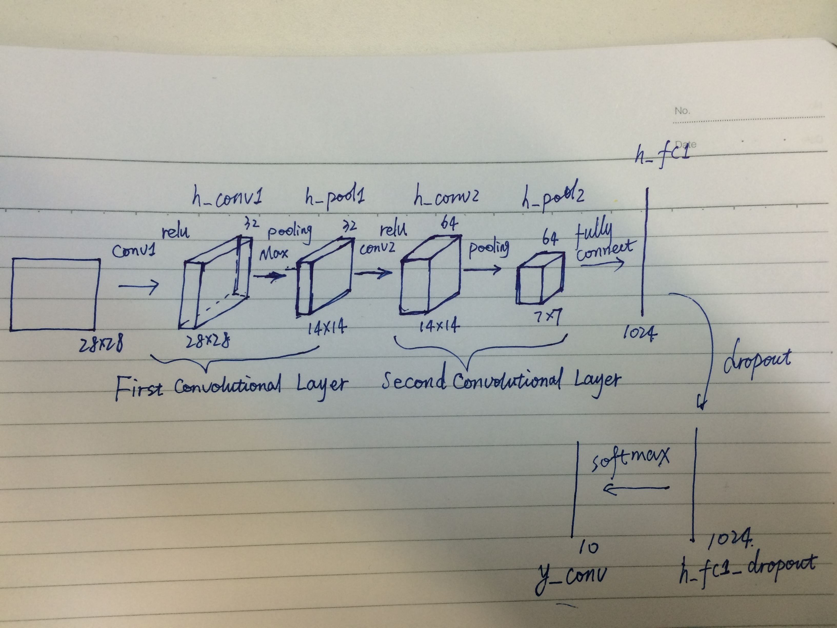
一、网络结构
二、代码
程序比较复杂,我就分成几个部分来叙述。
首先,下载并加载数据:
import tensorflow as tf
import tensorflow.examples.tutorials.mnist.input_data as input_data
mnist = input_data.read_data_sets("MNIST_data/", one_hot=True)     #下载并加载mnist数据
x = tf.placeholder(tf.float32, [None, 784])                        #输入的数据占位符
y_actual = tf.placeholder(tf.float32, shape=[None, 10])            #输入的标签占位符
定义四个函数,分别用于初始化权值W,初始化偏置项b, 构建卷积层和构建池化层。
为了建立这个模型,我们需要构建很多的权重和偏置值。人们通常初始化权重带有一定的噪声,主要是为了打破对称,且防止0梯度。既然这里我们使用了ReLU神经元,这个神经元对于初始化带有轻微积极的初始偏差,也可以算是一个比较好的经验实践。这里我们为了操作简单,不用重复去初始化操作,我们定义了几个函数如下:

#定义一个函数,用于初始化所有的权值 W
def weight_variable(shape):
  initial = tf.truncated_normal(shape, stddev=0.1)
  return tf.Variable(initial)

#定义一个函数,用于初始化所有的偏置项 b
def bias_variable(shape):
  initial = tf.constant(0.1, shape=shape)
  return tf.Variable(initial)
#对于卷积层,我们选择vanilla版本。我们的卷积使用步长为1且进行0填充操作,以保证输出和原输入size相同。
#定义一个函数,用于构建卷积层
def conv2d(x, W):
  return tf.nn.conv2d(x, W, strides=[1, 1, 1, 1], padding='SAME')
#Our pooling is plain old max pooling over 2x2 blocks .
#定义一个函数,用于构建池化层
def max_pool(x):
  return tf.nn.max_pool(x, ksize=[1, 2, 2, 1],strides=[1, 2, 2, 1], padding='SAME')
接下来构建网络。整个网络由两个卷积层(包含激活层和池化层),一个全连接层,一个dropout层和一个softmax层组成。
第一个卷积层:
The convolution will compute 32 features for each 5x5 patch.Its weight tensor will have a shape of [5, 5, 1, 32]. The first two dimensions are the patch size, the next is the number of input channels, and the last is the number of output channels.
w和b有多少组,卷积层结束后就输出多少层features map,也就是这里的output channels。一组w和b对应着一种卷积核,不同卷积核代表着关注的特征类别不同,用每种卷积核运算之后会得到一层特征图。
#构建网络
#在创建第一个卷积层之前,我们需要将输入数据x reshape成一个4维张量,其中的第2/3维对应着图像的width和height,最后一维对应着the number of color channels.
x_image = tf.reshape(x, [-1,28,28,1])         #转换输入数据shape,以便于用于网络中
W_conv1 = weight_variable([5, 5, 1, 32])
b_conv1 = bias_variable([32])
# convolve x_image with the weight tensor,add the bias, apply the ReLU function, and finally max pool.The max_pool_2x2 method
# will reduce the image size to 14x14.
h_conv1 = tf.nn.relu(conv2d(x_image, W_conv1) + b_conv1)     #第一个卷积层
h_pool1 = max_pool(h_conv1)                                  #第一个池化层
#In order to build a deep network, we stack several layers of this type. The second layer will have 64 features for each 5x5 patch
W_conv2 = weight_variable([5, 5, 32, 64])
b_conv2 = bias_variable([64])
h_conv2 = tf.nn.relu(conv2d(h_pool1, W_conv2) + b_conv2)      #第二个卷积层
h_pool2 = max_pool(h_conv2)                                   #第二个池化层
#Now that the image size has been reduced to 7x7, we add a fully-connected layer with 1024 neurons to allow processing on the
#entire image. We reshape the tensor from the pooling layer into a batch of vectors,multiply by a weight matrix, add a bias, and
# apply a ReLU.
W_fc1 = weight_variable([7 * 7 * 64, 1024])
b_fc1 = bias_variable([1024])
h_pool2_flat = tf.reshape(h_pool2, [-1, 7*7*64])              #reshape成向量
h_fc1 = tf.nn.relu(tf.matmul(h_pool2_flat, W_fc1) + b_fc1)    #第一个全连接层
#To reduce overfitting, we will apply dropout before readout layer. We create a placeholder for the probability that a neuron's
#output is kept during dropout. This allows us to turn dropout on during training, and turn it off during testing.
#TensorFlow's tf.nn.dropout op automatically handles scaling neuron outputs in addition to masking them , so dropout just works
#without any additional scaling.
keep_prob = tf.placeholder("float")
h_fc1_drop = tf.nn.dropout(h_fc1, keep_prob)                  #dropout层
#Finally,we add a layer,just like for the one layer softmax regression above.
W_fc2 = weight_variable([1024, 10])
b_fc2 = bias_variable([10])
y_predict=tf.nn.softmax(tf.matmul(h_fc1_drop, W_fc2) + b_fc2)   #softmax层
网络构建好后,就可以开始训练了。
大体和softmax模型一样。主要不同在于:
1·我们用更复杂的ADAM 优化器 取代了梯度下降。
2·我们在feed_dict部分添加了额外的参数keep_prob来控制dropout的比率。
3·我们在训练过程中的每100次迭代,将结果添加到日志。
cross_entropy = -tf.reduce_sum(y_actual*tf.log(y_predict))     #交叉熵
train_step = tf.train.GradientDescentOptimizer(1e-3).minimize(cross_entropy)    #梯度下降法
correct_prediction = tf.equal(tf.argmax(y_predict,1), tf.argmax(y_actual,1))
accuracy = tf.reduce_mean(tf.cast(correct_prediction, "float"))                 #精确度计算
sess=tf.InteractiveSession()
sess.run(tf.initialize_all_variables())
for i in range(20000):
  batch = mnist.train.next_batch(50)
  if i%100 == 0:                  #训练100次,验证一次
    train_acc = accuracy.eval(feed_dict={x:batch[0], y_actual: batch[1], keep_prob: 1.0})
    print 'step %d, training accuracy %g'%(i,train_acc)
    train_step.run(feed_dict={x: batch[0], y_actual: batch[1], keep_prob: 0.5})

test_acc=accuracy.eval(feed_dict={x: mnist.test.images, y_actual: mnist.test.labels, keep_prob: 1.0})
print "test accuracy %g"%test_acc
Tensorflow依赖于一个高效的C++后端来进行计算。与后端的这个连接叫做session。一般而言,使用TensorFlow程序的流程是先创建一个图,然后在session中启动它。
这里,我们使用更加方便的InteractiveSession类。通过它,你可以更加灵活地构建你的代码。它能让你在运行图的时候,插入一些计算图,这些计算图是由某些操作(operations)构成的。这对于工作在交互式环境中的人们来说非常便利,比如使用IPython。
训练20000次后,再进行测试,测试精度可以达到99%。
完整代码:

# -*- coding: utf-8 -*-
"""
Created on Thu Sep  8 15:29:48 2016

@author: root
"""
import tensorflow as tf
#导入input_data用于自动下载和安装MNIST数据集
import tensorflow.examples.tutorials.mnist.input_data as input_data
mnist = input_data.read_data_sets("MNIST_data/", one_hot=True) #下载并加载mnist数据
#创建两个占位符,x为输入网络的图像,y_为输入网络的图像类别
x = tf.placeholder(tf.float32, [None, 784])                        #输入的数据占位符
y_actual = tf.placeholder(tf.float32, shape=[None, 10])            #输入的标签占位符

#定义一个函数,用于初始化所有的权值 W
def weight_variable(shape):
  #输出服从截尾正态分布的随机值
  initial = tf.truncated_normal(shape, stddev=0.1)
  return tf.Variable(initial)

#定义一个函数,用于初始化所有的偏置项 b
def bias_variable(shape):
  initial = tf.constant(0.1, shape=shape)
  return tf.Variable(initial)

#定义一个函数,用于构建卷积层
#x 是一个4维张量,shape为[batch,height,width,channels]
#卷积核移动步长为1。填充类型为SAME,可以不丢弃任何像素点
def conv2d(x, W):
  return tf.nn.conv2d(x, W, strides=[1, 1, 1, 1], padding='SAME')

#定义一个函数,用于构建池化层
#采用最大池化,也就是取窗口中的最大值作为结果
#x 是一个4维张量,shape为[batch,height,width,channels]#ksize表示pool窗口大小为2x2,也就是高2,宽2
#strides,表示在height和width维度上的步长都为2
def max_pool(x):
  return tf.nn.max_pool(x, ksize=[1, 2, 2, 1],strides=[1, 2, 2, 1], padding='SAME')

#构建网络
#把输入x(二维张量,shape为[batch, 784])变成4d的x_image,x_image的shape应该是[batch,28,28,1]
#-1表示自动推测这个维度的size,表示一次输入计算的数量
x_image = tf.reshape(x, [-1,28,28,1])         #转换输入数据shape,以便于用于网络中
#初始化W为[5,5,1,32]的张量,表示卷积核大小为5*5,第一层网络的输入和输出神经元个数分别为1和32
W_conv1 = weight_variable([5, 5, 1, 32])
#初始化b为[32],即输出大小
b_conv1 = bias_variable([32])
#把x_image和权重进行卷积,加上偏置项,然后应用ReLU激活函数,最后进行max_pooling
#h_pool1的输出即为第一层网络输出,shape为[batch,14,14,1]
h_conv1 = tf.nn.relu(conv2d(x_image, W_conv1) + b_conv1)     #第一个卷积层
h_pool1 = max_pool(h_conv1)                                  #第一个池化层
#第2层,卷积层
#卷积核大小依然是5*5,这层的输入和输出神经元个数为32和64
W_conv2 = weight_variable([5, 5, 32, 64])
b_conv2 = bias_variable([64])
#h_pool2即为第二层网络输出,shape为[batch,7,7,1]
h_conv2 = tf.nn.relu(conv2d(h_pool1, W_conv2) + b_conv2)      #第二个卷积层
h_pool2 = max_pool(h_conv2)                                   #第二个池化层
#第3层, 全连接层
#这层是拥有1024个神经元的全连接层
#W的第1维size为7*7*64,7*7是h_pool2输出的size,64是第2层输出神经元个数
W_fc1 = weight_variable([7 * 7 * 64, 1024])
b_fc1 = bias_variable([1024])
#计算前需要把第2层的输出reshape成[batch, 7*7*64]的张量
h_pool2_flat = tf.reshape(h_pool2, [-1, 7*7*64])        #reshape成向量-1代表的含义是不用我们自己指定这一维的大小,函数会自动算,
h_fc1 = tf.nn.relu(tf.matmul(h_pool2_flat, W_fc1) + b_fc1)    #第一个全连接层
#Dropout层
#为了减少过拟合,在输出层前加入dropout
keep_prob = tf.placeholder("float")
h_fc1_drop = tf.nn.dropout(h_fc1, keep_prob)                  #dropout层
#输出层
#最后,添加一个softmax层
#可以理解为另一个全连接层,只不过输出时使用softmax将网络输出值转换成了概率
W_fc2 = weight_variable([1024, 10])
b_fc2 = bias_variable([10])
y_predict=tf.nn.softmax(tf.matmul(h_fc1_drop, W_fc2) + b_fc2)   #softmax层
#预测值和真实值之间的交叉墒
cross_entropy = -tf.reduce_sum(y_actual*tf.log(y_predict))     #交叉熵
#train op, 使用ADAM优化器来做梯度下降。学习率为0.0001
train_step = tf.train.GradientDescentOptimizer(1e-3).minimize(cross_entropy)    #梯度下降法
#评估模型,tf.argmax能给出某个tensor对象在某一维上数据最大值的索引。
#因为标签是由0,1组成了one-hot vector,返回的索引就是数值为1的位置
correct_prediction = tf.equal(tf.argmax(y_predict,1), tf.argmax(y_actual,1))
#计算正确预测项的比例,因为tf.equal返回的是布尔值,
#使用tf.cast把布尔值转换成浮点数,然后用tf.reduce_mean求平均值
accuracy = tf.reduce_mean(tf.cast(correct_prediction, "float"))                 #精确度计算
#创建一个交互式Session
sess=tf.InteractiveSession()
#初始化变量
sess.run(tf.initialize_all_variables())
#开始训练模型,循环20000次,每次随机从训练集中抓取50幅图像
for i in range(20000):
  batch = mnist.train.next_batch(50)
  if i%100 == 0:                  #训练100次,验证一次
    #每100次输出一次日志
    train_acc = accuracy.eval(feed_dict={x:batch[0], y_actual: batch[1], keep_prob: 1.0})
    print('step',i,'training accuracy',train_acc)
    train_step.run(feed_dict={x: batch[0], y_actual: batch[1], keep_prob: 0.5})

test_acc=accuracy.eval(feed_dict={x: mnist.test.images, y_actual: mnist.test.labels, keep_prob: 1.0})
print("test accuracy",test_acc)
最终测试集上的准确率大概是99.2%


 4745
4745


 被折叠的 条评论
为什么被折叠?
被折叠的 条评论
为什么被折叠?
 到【灌水乐园】发言


