Faster R-CNN的理解

前提

目标检测第一代算法R-CNN，第二代是Fast R-CNN ，第三代是Faster R-CNN，目标检测区域卷积神经网络一代比一代速度快且强。
Faster R-CNN论文：
《Faster R-CNN: Towards Real-Time Object Detection with Region Proposal Networks》
读论文可以了解其思想，为我们提供了一种解决问题的思路，通过读论文有了一些自己浅显的理解，仅此记录一下

论文

Abstract

state-of-the-art object detection networks depend on region proposal algorithms to hypothesize object locations. Advances like SPPnet and Fast R-CNN have reduced the running time of these detection networks, exposing region proposal computation as a bottleneck. In this work, we introduce a Region Proposal Network (RPN) that shares full-image convolutional features with the detection network, thus enabling nearly cost-free region proposals. An RPN is a fully convolutional network that simultaneously predicts object bounds and objectness scores at each position. The RPN is trained end-to-end to generate high-quality region proposals, which are used by Fast R-CNN for detection. We further merge RPN and Fast R-CNN into a single network by sharing their convolutional features—using the recently popular terminology of neural networks with ‘attention’ mechanisms, the RPN component tells the unified network where to look. For the very deep VGG-16 model, our detection system has a frame rate of 5fps (including all steps) on a GPU, while achieving state-of-the-art object detection accuracy on PASCAL VOC 2007, 2012, and MS COCO datasets with only 300 proposals per image. In ILSVRC and COCO 2015 competitions, Faster R-CNN and RPN are the foundations of the 1st-place winning entries in several tracks. Code has been made publicly available.

摘要

摘要主要有几点内容：

• 在这篇论文之前，目标检测都是用区域提议算法来假设目标位置。
• 引入了一种RPN网络，对区域提议基本上没有时间的消耗
• RPN是全卷积网络结构，可同时预测目标边框和目标得分
• 在GPU上达到了5帧的效果
• 代码公开可以自己复现

1. Introduction

Recent advances in object detection are driven by the success of region proposal methods (e.g., [4]) and region-based convolutional neural networks (R-CNNs) [5]. Although region-based CNNs were computationally expensive as originally developed in [5], their cost has been drastically reduced thanks to sharing convolutions across proposals [1], [2]. The latest incarnation, Fast R-CNN [2], achieves near real-time rates using very deep networks [3], when ignoring the time spent on region proposals. Now, proposals are the test-time computational bottleneck in state-of-the-art detection systems.

• 这篇论文之前，提取框是最大的计算瓶颈，后面需要解决这个事。

Region proposal methods typically rely on inexpensive features and economical inference schemes. Selective Search [4], one of the most popular methods, greedily merges superpixels based on engineered low-level features. Yet when compared to efficient detection networks [2], Selective Search is an order of magnitude slower, at 2 seconds per image in a CPU implementation. EdgeBoxes[6] currently provides the best tradeoff between proposal quality and speed, at 0.2 seconds per image. Nevertheless, the region proposal step still consumes as much running time as the detection network.

• 之前的提取框使用Selective Search方法做的，但这种方法只能在cpu上做，所以相比GPU会非常的耗时，光单张图像就有2秒，很慢。
• Selective Search 为什么不能用GPU? 因为它既不是一个网络也不是什么架构，只是用传统基本的算法来提取候选框。

One may note that fast region-based CNNs take advantage of GPUs, while the region proposal methods used in research are implemented on the CPU, making such runtime comparisons inequitable. An obvious way to accelerate proposal computation is to re-implement it for the GPU. This may be an effective engineering solution, but re-implementation ignores the down-stream detection network and therefore misses important opportunities for sharing computation.

• 这时就有了改进的思想，能不能改改放到GPU算，这样计算肯定会快，瓶颈也就解决了

In this paper, we show that an algorithmic change—computing proposals with a deep convolutional neural network—leads to an elegant and effective solution where proposal computation is nearly cost-free given the detection network’s computation. To this end, we introduce novel Region Proposal Networks (RPNs) that share convolutional layers with state-of-the-art object detection networks[1],[2] . By sharing convolutions at test-time, the marginal cost for computing proposals is small (e.g., 10ms per image).

• 接着就是论文的核心了，引入了RPN网络，让它在GPU上工作提取候选框以及之后的事情。

Our observation is that the convolutional feature maps used by region-based detectors, like Fast R-CNN, can also be used for generating region proposals. On top of these convolutional features, we construct an RPN by adding a few additional convolutional layers that simultaneously regress region bounds and objectness scores at each location on a regular grid. The RPN is thus a kind of fully convolutional network (FCN)[7] and can be trained end-to-end specifically for the task for generating detection proposals.

• 这个RPN是由一些卷积层组成的
• 用这个RPN来做两件事情，一件是判断是不是目标物体，是物体就是前景，不是物体就是背景，用来进行分类，也就是二分类任务;第二件事就是搞这个候选框了，要把框移动合适的位置，这就成了一个回归任务。
• 这样一分析，RPN就是两个分支走，一个是对候选框搞回归的，另一分支判断是不是物体，走分类路线。RPN只有卷积层没有全连接层，所以它是一个全卷积网络FCN （如CNN去掉全连接层就成了FCN）。
  
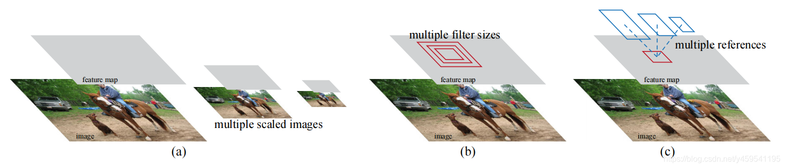
  Figure 1: Different schemes for addressing multiple scales and sizes. (a) Pyramids of images and feature maps are built, and the classifier is run at all scales. (b) Pyramids of filters with multiple scales/sizes are run on the feature map. © We use pyramids of reference boxes in the regression functions.

RPNs are designed to efficiently predict region proposals with a wide range of scales and aspect ratios. In contrast to prevalent methods [8], [9], [1], [2] that use pyramids of images (Figure 1, a) or pyramids of filters (Figure 1, b), we introduce novel “anchor” boxes that serve as references at multiple scales and aspect ratios. Our scheme can be thought of as a pyramid of regression references (Figure 1, c), which avoids enumerating images or filters of multiple scales or aspect ratios. This model performs well when trained and tested using single-scale images and thus benefits running speed.

• 提出了一种“锚”的方法用来解决多尺度和尺寸大小问题，这种方法可以从图像中提取大小不同的候选框，解决了即想检测图像中的大物体，同时也想检测图像中小物体的问题。
• （Figure 1,a)中做法是把图像resize，这样提取的框就有大有小了，这是图像金字塔方法。一张图变成不同大小的多张图输入，虽然大物体小物体都可以找到但速度慢，效率低。
• （Figure 1, b)中的做法和a不一样了，不对图像操作变换了，改成对图像的feature做不同大小的变换，这种也是大大增加了计算量，速度会非常的慢。

To unify RPNs with Fast R-CNN [2] object detection networks, we propose a training scheme that alternates between fine-tuning for the region proposal task and then fine-tuning for object detection, while keeping the proposals fixed. This scheme converges quickly and produces a unified network with convolutional features that are shared between both tasks.
We comprehensively evaluate our method on the PASCAL VOC detection benchmarks [11] where RPNs with Fast R-CNNs produce detection accuracy better than the strong baseline of Selective Search with Fast R-CNNs. Meanwhile, our method waives nearly all computational burdens of Selective Search at test-time——the effective running time for proposals is just 10 milliseconds. Using the expensive very deep models of [3], our detection method still has a frame rate of 5fps (including all steps) on a GPU, and thus is a practical object detection system in terms of both speed and accuracy. We also report results on the MS COCO dataset [12] and investigate the improvements on PASCAL VOC using the COCO data. Code has been made publicly available at https://github.com/shaoqingren/faster_rcnn (in MATLAB) and https://github.com/rbgirshick/py-faster-rcnn (in Python).

• 使用锚点这种检测方法，在GPU上的帧率有5fps。比之前传统的快了好多。

A preliminary version of this manuscript was published previously [10]. Since then, the frameworks of RPN and Faster R-CNN have been adopted and generalized to other methods, such as 3D object detection [13], part-based detection [14], instance segmentation [15], and image captioning [16]. Our fast and effective object detection system has also been built in commercial systems such as at Pinterests [17], with user engagement improvements reported.
In ILSVRC and COCO 2015 competitions, Faster R-CNN and RPN are the basis of several 1st-place entries [18] in the tracks of ImageNet detection, ImageNet localization, COCO detection, and COCO segmentation. RPNs completely learn to propose regions from data, and thus can easily benefit from deeper and more expressive features (such as the 101-layer residual nets adopted in [18]). Faster R-CNN and RPN are also used by several other leading entries in these competitions. These results suggest that our method is not only a cost-efficient solution for practical usage, but also an effective way of improving object detection accuracy.

• Faster R-CNN能检测好多东西，也有了商业化应用。

2. RELATED WORK

略～

3. FASTER R-CNN

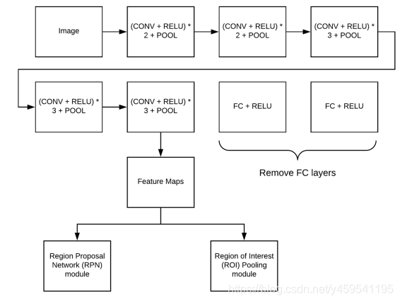
Our object detection system, called Faster R-CNN, is composed of two modules. The first module is a deep fully convolutional network that proposes regions, and the second module is the Fast R-CNN detector [2] that uses the proposed regions. The entire system is a single, unified network for object detection (Figure 2). Using the recently popular terminology of neural networks with attention [31] mechanisms, the RPN module tells the Fast R-CNN module where to look. In Section 3.1 we introduce the designs and properties of the network for region proposal. In Section 3.2 we develop algorithms for training both modules with features shared.

Figure 2: Faster R-CNN is a single, unified network for object detection. The RPN module serves as the ‘attention’ of this unified network.

• Faster R-CNN的整体网络结构是有两部分组成的。
• 第一部分是深度全卷积网络
• 第二部分是Fast R-CNN检测器

3.1 Region Proposal Networks

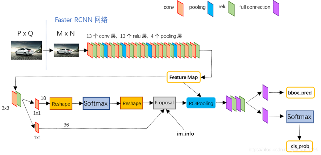
A Region Proposal Network (RPN) takes an image (of any size) as input and outputs a set of rectangular object proposals, each with an objectness score 3. We model this process with a fully convolutional network [7], which we describe in this section. ==Because our ultimate goal is to share computation with a Fast R-CNN object detection network ==[2], we assume that both nets share a common set of convolutional layers. In our experiments, we investigate the Zeiler and Fergus model 32, which has 5 shareable convolutional layers and the Simonyan and Zisserman model 3, which has 13 shareable convolutional layers.

• RPN网络可以把一张任意大小的图像作为输入，没有了尺寸的限制，很方便，以前是所有的图像必须是同等大小的。
• RPN 网络的输出是一系列的候选框
• 经过RPN 网络得到的是当前物体的框，以及这个框里是不是物体的得分（不是
  ----物体属于哪个类别的得分）。
• 最终目标是想与Fast R-CNN共享卷积计算的。end2end的模式，输入一张图像直接跑卷积，来共享卷积计算。

To generate region proposals, we slide a small network over the convolutional feature map output by the last shared convolutional layer. This small network takes as input an n×n spatial window of the input convolutional feature map. Each sliding window is mapped to a lower-dimensional feature (256-d for ZF and 512-d for VGG, with ReLU [33] following). This feature is fed into two sibling fully-connected layers——a box-regression layer (reg) and a box-classification layer (cls). We use n=3 in this paper, noting that the effective receptive field on the input image is large (171 and 228 pixels for ZF and VGG, respectively). This mini-network is illustrated at a single position in Figure 3 (left). Note that because the mini-network operates in a sliding-window fashion, the fully-connected layers are shared across all spatial locations. This architecture is naturally implemented with an n×n convolutional layer followed by two sibling 1 × 1 convolutional layers (for reg and cls, respectively).

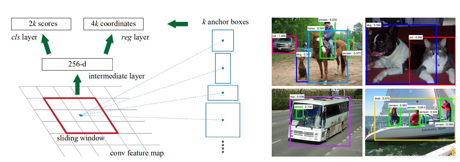
Figure 3: Left: Region Proposal Network (RPN). Right: Example detections using RPN proposals on PASCAL VOC 2007 test.Our method detects objects in a wide range of scales and aspect ratios.

3.1.1 Anchors

At each sliding-window location, we simultaneously predict multiple region proposals, where the number of maximum possible proposals for each location is denoted as k. So the reg layer has 4k outputs encoding the coordinates of k boxes, and the cls layer outputs 2k scores that estimate probability of object or not object for each proposal. The k proposals are parameterized relative to k reference boxes, which we call anchors. An anchor is centered at the sliding window in question, and is associated with a scale and aspect ratio (Figure 3, left). By default we use 3 scales and 3 aspect ratios, yielding k=9 anchors at each sliding position. For a convolutional feature map of a size W × H (typically ∼2,400), there are WHk anchors in total.

• 为了生成这个候选框，做了一件事情，就是在卷积特征图上搞了一个滑动窗口（n=3,也就是窗口大小为3x3），用这个滑动窗口再做一次卷积
• 如图3,feature map上用滑动窗口卷积，我们知道做卷积之后得到的还是特征图，特征图上的点映射到原始图像上就成了区域，这就是感受野
• 特征图上每个“点”对应原图中有k个区域框，目的在上面说过，每个框判断是不是物体以及每个框对对应的坐标
• 每个特征点有k（k=9）个不同尺度和比例大小的框，这样区域就会有很多很多
• 为了覆盖检测物体更加的多，检测精度高一些，同时也要保证时间效率，对k个anchor box采取了一种策略：3种不同尺寸的比例和3种不同基准的大小。长宽比h:w有1：2， 2：1， 1：1，这个比例是初始的比例后面是要计算调整的不是最终框选物体结果的比例，而基准大小：128x128, 256x256, 512x512。
• 总之就是说，对于特征图上的一个点，映射到原始图像上的框 。通过feature map点感受野的位置和感受野的大小，就能得到对应原始图像上对应的框，也就是说这个框可以覆盖到图像中的任何位置。获得这些框做什么呢，对于每个框在这时走两条路，一条通往分类，进行分类判断，判断一下这个框当前是不是一个物体；另一条路通往回归，计算回归值与ground truth值之间的差异。
• 2k score -----表示对于每一种框可以知道不是物体的得分和是物体的得分，是前景还是背景的二分类，也就是对每种框都做一个二分类，一共有9种框（k=9），2k就是18个结果得分。
• 4k score -----4k就是36，对于一种框有x,y,h,w,四个值，坐标的回归值。
• 如果特征图的大小为W×H，那就需要W×H×K个anchor。文中的2400个特征点是在CNN最后一层（conv5）得出的40×60大小的特征图（每个特征图上的点都用到了，乘以下是2400）。所有特征点（每个点对应9种框）映射原始图像的anchor（框）数量也就是40×60×9约等于2w个。框太多了就需要过滤一下

Translation-Invariant Anchors

An important property of our approach is that it is translation invariant, both in terms of the anchors and the functions that compute proposals relative to the anchors. If one translates an object in an image, the proposal should translate and the same function should be able to predict the proposal in either location. This translation-invariant property is guaranteed by our method. As a comparison, the MultiBox method [27] uses k-means to generate 800 anchors, which are not translation invariant. So MultiBox does not guarantee that the same proposal is generated if an object is translated.

• 锚点的平移不变性，比如在一张图像（上图所示）中有个长方形物体a，它原来在图像的左边可以检测到，当把它移到图像右边了（绿色a）也能检测到。因为图像中会产生很多个框，总有一个框能把物体a正确框出来的。

Multi-Scale Anchors as Regression References

Our design of anchors presents a novel scheme for addressing multiple scales (and aspect ratios). As shown in Figure 1, there have been two popular ways for multi-scale predictions. The first way is based on image/feature pyramids, e.g., in DPM [8] and CNN-based methods [9], [1], [2]. The images are resized at multiple scales, and feature maps (HOG [8] or deep convolutional features [9], [1], [2]) are computed for each scale (Figure 1(a)). This way is often useful but is time-consuming. The second way is to use sliding windows of multiple scales (and/or aspect ratios) on the feature maps. For example, in DPM [8], models of different aspect ratios are trained separately using different filter sizes (such as 5×7 and 7×5). If this way is used to address multiple scales, it can be thought of as a “pyramid of filters” (Figure 1(b)). The second way is usually adopted jointly with the first way [8].

As a comparison, our anchor-based method is built on a pyramid of anchors, which is more cost-efficient. Our method classifies and regresses bounding boxes with reference to anchor boxes of multiple scales and aspect ratios. It only relies on images and feature maps of a single scale, and uses filters (sliding windows on the feature map) of a single size. We show by experiments the effects of this scheme for addressing multiple scales and sizes (Table 8).

Because of this multi-scale design based on anchors, we can simply use the convolutional features computed on a single-scale image, as is also done by the Fast R-CNN detector [2]. The design of multi-scale anchors is a key component for sharing features without extra cost for addressing scales.

• 通过比较，anchor方法比较节省时间
• 共享特征的关键是多尺度锚点的设计使用，多尺度锚点是RPN 网络的核心组成

3.1.2 Loss Function

For training RPNs, we assign a binary class label (of being an object or not) to each anchor. We assign a positive label to two kinds of anchors: (i) the anchor/anchors with the highest Intersection-over-Union (IoU) overlap with a ground-truth box, or (ii) an anchor that has an IoU overlap higher than 0.7 with any ground-truth box. Note that a single ground-truth box may assign positive labels to multiple anchors. Usually the second condition is sufficient to determine the positive samples; but we still adopt the first condition for the reason that in some rare cases the second condition may find no positive sample. We assign a negative label to a non-positive anchor if its IoU ratio is lower than 0.3 for all ground-truth boxes. Anchors that are neither positive nor negative do not contribute to the training objective.

• IoU-----预测的框（如上图红色框）与真实物体的边界框（绿色框）重叠的越多越好，这样IoU的得分越高。

• 做一个二分类的标签，看当前的框是一个物体或者不是一个物体

• 两种方法贴正标签：一种是具有与实际边界框的重叠最高交并比（IoU）的锚点；第二种是具有与实际边界框的重叠超过0.7 IoU的锚点。

• 贴负标签：锚点的IoU比率低于0.3

With these definitions, we minimize an objective function following the multi-task loss in Fast R-CNN [2]. Our loss function for an image is defined as:

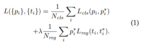
Here, i is the index of an anchor in a mini-batch and p_i is the predicted probability of anchor i being an object. The ground-truth label p*_i is 1 if the anchor is positive, and is 0 if the anchor is negative. t_i is a vector representing the 4 parameterized coordinates of the predicted bounding box, and t*_i is that of the ground-truth box associated with a positive anchor. The classification loss L_cls is log loss over two classes (object vs not object). For the regression loss, we use L_reg(t_i,t*_i)=R(t_i−t*_i) where R is the robust loss function (smooth L₁) defined in [2]. The term p*_i L_reg means the regression loss is activated only for positive anchors (p*_i=1) and is disabled otherwise (p*_i=0). The outputs of the cls and reg layers consist of {p_i} and {t_i} respectively.

• i是anchor的索引，p_i是锚点i作为目标的预测概率，p*_i为1时是正例，为0是负例，t_i是预测边界框4个参数化坐标的向量，t*_i是与正锚点相关的真实边界框的向量，L_cls是两个类别上（目标或不是目标）的对数损失，回归损失是L_reg
• 一个框是物体了，对回归进行微调，若不是物体p*_i=0，没有必要对L_reg微调，后一项直接为零

The two terms are normalized by Ncls and Nreg and weighted by a balancing parameter λ. In our current implementation (as in the released code), the cls term in Eqn.(1) is normalized by the mini-batch size (ie, N_cls=256) and the reg term is normalized by the number of anchor locations (ie, N_reg∼2,400). By default we set λ=10, and thus both cls and reg terms are roughly equally weighted. We show by experiments that the results are insensitive to the values of λ in a wide range(Table 9). We also note that the normalization as above is not required and could be simplified.

• λ值是一个权衡值，越大就是越倾向与回归损失函数，重视回归，反之倾向于分类

For bounding box regression, we adopt the parameterizations of the 4 coordinates following [5]:

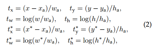
where x, y, w, and h denote the box’s center coordinates and its width and height. Variables x, x_a, and x* are for the predicted box, anchor box, and ground-truth box respectively (likewise for y,w,h). This can be thought of as bounding-box regression from an anchor box to a nearby ground-truth box.

Nevertheless, our method achieves bounding-box regression by a different manner from previous RoI-based (Region of Interest) methods [1], [2]. In [1], [2], bounding-box regression is performed on features pooled from arbitrarily sized RoIs, and the regression weights are shared by all region sizes. In our formulation, the features used for regression are of the same spatial size (3 × 3) on the feature maps. To account for varying sizes, a set of k bounding-box regressors are learned. Each regressor is responsible for one scale and one aspect ratio, and the k regressors do not share weights. As such, it is still possible to predict boxes of various sizes even though the features are of a fixed size/scale, thanks to the design of anchors.

• 用于回归的特征计算，使用均是3×3卷积核
• 锚点的这种设计方法，可以预测各种尺寸的框。

3.1.3 Training RPNs

The RPN can be trained end-to-end by back-propagation and stochastic gradient descent (SGD) [35]. We follow the “image-centric” sampling strategy from [2] to train this network. Each mini-batch arises from a single image that contains many positive and negative example anchors. It is possible to optimize for the loss functions of all anchors, but this will bias towards negative samples as they are dominate. Instead, we randomly sample 256 anchors in an image to compute the loss function of a mini-batch, where the sampled positive and negative anchors have a ratio of up to 1:1. If there are fewer than 128 positive samples in an image, we pad the mini-batch with negative ones.

• RPN 训练是end to end
• 用了SGD优化器
• 训练过程是一张图像一张图像input做的，每次迭代训练一张图
• 在一张图像中随机选取256个
• 尽量让正负样本1：1，若正样本不够拿负样本填充

We randomly initialize all new layers by drawing weights from a zero-mean Gaussian distribution with standard deviation 0.01. All other layers (i.e., the shared convolutional layers) are initialized by pre-training a model for ImageNet classification [36], as is standard practice [5]. We tune all layers of the ZF net, and conv3_1 and up for the VGG net to conserve memory [2]. We use a learning rate of 0.001 for 60k mini-batches, and 0.0001 for the next 20k mini-batches on the PASCAL VOC dataset. We use a momentum of 0.9 and a weight decay of 0.0005 [37]. Our implementation uses Caffe [38].

• 用高斯初始化，标准差为0.01

3.2 Sharing Features for RPN and Fast R-CNN

略。。。

3.3 Implementation Details

We train and test both region proposal and object detection networks on images of a single scale [1], [2]. We re-scale the images such that their shorter side is s=600 pixels [2]. Multi-scale feature extraction (using an image pyramid) may improve accuracy but does not exhibit a good speed-accuracy trade-off [2]. On the re-scaled images, the total stride for both ZF and VGG nets on the last convolutional layer is 16 pixels, and thus is ∼10 pixels on a typical PASCAL image before resizing (∼500×375). Even such a large stride provides good results, though accuracy may be further improved with a smaller stride.
For anchors, we use 3 scales with box areas of 128², 256², and 512² pixels, and 3 aspect ratios of 1:1, 1:2, and 2:1. These hyper-parameters are not carefully chosen for a particular dataset, and we provide ablation experiments on their effects in the next section. As discussed, our solution does not need an image pyramid or filter pyramid to predict regions of multiple scales, saving considerable running time. Figure 3 (right) shows the capability of our method for a wide range of scales and aspect ratios. Table 1 shows the learned average proposal size for each anchor using the ZF net. We note that our algorithm allows predictions that are larger than the underlying receptive field. Such predictions are not impossible—one may still roughly infer the extent of an object if only the middle of the object is visible.

• 预处理输入图像，调整输入图像短边为600，比例保持不变

The anchor boxes that cross image boundaries need to be handled with care. During training, we ignore all cross-boundary anchors so they do not contribute to the loss. For a typical 1000×600 image, there will be roughly 20000 (≈60×40×9) anchors in total. With the cross-boundary anchors ignored, there are about 6000 anchors per image for training. If the boundary-crossing outliers are not ignored in training, they introduce large, difficult to correct error terms in the objective, and training does not converge. During testing, however, we still apply the fully convolutional RPN to the entire image. This may generate cross-boundary proposal boxes, which we clip to the image boundary.

Some RPN proposals highly overlap with each other. To reduce redundancy, we adopt non-maximum suppression (NMS) on the proposal regions based on their cls scores. We fix the IoU threshold for NMS at 0.7, which leaves us about 2000 proposal regions per image. As we will show, NMS does not harm the ultimate detection accuracy, but substantially reduces the number of proposals. After NMS, we use the top-N ranked proposal regions for detection. In the following, we train Fast R-CNN using 2000 RPN proposals, but evaluate different numbers of proposals at test-time.

• 训练时，越界框直接过滤到，剩6000个框
• 测试时，越界框剪切到图像边界
• 6000个框还是有点多了，采取非极大值抑制（NMS）过滤框，筛选后每张图像留下了大约2000个框
• 在NMS之后，按得分排序，取top-N，如取前256个框训练网络。

4. EXPERIMENTS

略。。。

5. CONCLUSION

We have presented RPNs for efficient and accurate region proposal generation. By sharing convolutional features with the down-stream detection network, the region proposal step is nearly cost-free. Our method enables a unified, deep-learning-based object detection system to run at near real-time frame rates. The learned RPN also improves region proposal quality and thus the overall object detection accuracy.

• 总结了一下，主要是提出了RPN网络，共享了卷积，近乎实时帧率运行，在精度保证下，速度比上一代提高了好多 。

总结:Faster R-CNN

1.Faster R-CNN整体框架

• Faster R-CNN = Fast R-CNN + RPN
• 不再采用Selective Search模块（包括Fast R-CNN以前，都是采用Selective Search），性能得到大大提升
• 共享了卷积层计算
• 用了Attention 注意机制，目的是引导Fast R-CNN关注区域
• 区域候选框（Region Proposals）是量少质优（~300/image）
• 4种losses：

1. RPN classify object /not object
2. RPN regress box coordinates
3. Final classification score(object classes)
4. Final box coordinates

2.Region Proposal Network（RPN）网络

• RPN是Faster R-CNN 的核心
• 是一个全卷积网络（FCN）
• 引入了Anchor：3个尺度（128², 256², 512²）和3个长宽比（1:1，1:2，2:1）
• 特征图大小WH，Anchor数量WH*K
  

3.训练流程（4步）

• 第1步：训练RPN网络

  • ImageNet的预训练模型对卷积层进行初始化（卷积层没有共享）

• 第2步：训练Fast R-CNN网络

  • 由第1步RPN生成的候选框，单独训练Fast R-CNN网络，对其卷积层进行初始化（卷积层没有共享）

• 第3步：调优RPN

  • 由Fast R-CNN网络的卷积层参数来初始化RPN训练
  • 固定共享卷积层，只对RPN进行微调 （卷积层共享）

• 第4步：调优Fast R-CNN

  • 区域候选框是由第3步的RPN生成的
  • 保持共享卷积层的固定，对Fast R-CNN进行微调 （卷积层共享）

4.Faster R-CNN 性能和速度对比

	Faster R-CNN	Fast R-CNN	R-CNN
单图测试时间	0.198s	2.0s	50.0s
PASCAL VOC 07 mAP	66.9%	66.9%	66.0%

Reference：
https://cloud.tencent.com/developer/news/281788
https://blog.csdn.net/quincuntial/article/details/79132243
https://www.jianshu.com/p/ab1ebddf58b1
https://arxiv.org/abs/1506.01497
https://www.pyimagesearch.com/deep-learning-computer-vision-python-book/
https://www.cnblogs.com/wangyong/p/8513563.html
https://www.cnblogs.com/zyly/p/9247863.html