数据分析--分类与回归模型（一）

最新推荐文章于 2024-08-15 14:17:41 发布

yili_sha11

最新推荐文章于 2024-08-15 14:17:41 发布

阅读量9.3k

点赞数 6

分类专栏：数据分析文章标签：数据分析--分类与回归模型（一）

本文链接：https://blog.csdn.net/yili_sha11/article/details/100062327

版权

数据分析专栏收录该内容

6 篇文章 0 订阅

订阅专栏

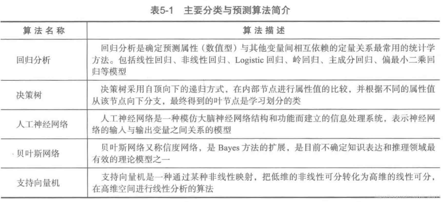
一、分类回归方法

主要的分类、回归算法，网上和书上的资料进行梳理整理。

二、各类分类方法

代码参照《人工智能：python实现》一书，对部分代码进行了修改。

1、logistic 回归

logistics回归模型步骤

根据挖掘目的设置特征，并筛选特征x1，x2...xp,使用sklearn中的feature_selection库，F检验来给出特征的F值和P值，筛选出F大的，p小的值。RFE（递归特征消除）和SS（稳定性选择）
列出回归方程ln（p/1-p）=β0+β1x1+...+βpxp+e
估计回归系数
模型检验
预测控制

import numpy as np
from sklearn import linear_model
import matplotlib.pyplot as plt

from utilities import visualize_classifier

# Define sample input data
X = np.array([[3.1, 7.2], [4, 6.7], [2.9, 8], [5.1, 4.5], [6, 5], [5.6, 5], [3.3, 0.4], [3.9, 0.9], [2.8, 1], [0.5, 3.4], [1, 4], [0.6, 4.9]])
y = np.array([0, 0, 0, 1, 1, 1, 2, 2, 2, 3, 3, 3])
test=np.array([[3.5,6.7],[4.2,5.5]])
help(linear_model.LogisticRegression)
# Create the logistic regression classifier
clf = linear_model.LogisticRegression(solver='liblinear', C=1) #C为惩罚系数，过大易过拟合
#LogisticRegression(penalty='l2', dual=False, tol=0.0001, C=1.0, fit_intercept=True, intercept_scaling=1, class_weight=None, random_state=None, solver='warn', max_iter=100, multi_class='warn', verbose=0, warm_start=False, n_jobs=None, l1_ratio=None)

# Train the classifier
clf.fit(X, y)
#输出所有相关参数
print(clf.classes_) #输出分类类别
print(clf.coef_) #输出分类回归系数
print(clf.intercept_) #截距
print(clf.n_iter_) #输出迭代次数
print(clf.score(X,y))
y_pred=clf.predict(test) #预测数据
print(y_pred)

#图形化输出
def visualize_classifier(classifier, X, y):
# Define the minimum and maximum values for X and Y
# that will be used in the mesh grid
min_x, max_x = X[:, 0].min() - 1.0, X[:, 0].max() + 1.0
min_y, max_y = X[:, 1].min() - 1.0, X[:, 1].max() + 1.0

# Define the step size to use in plotting the mesh grid
mesh_step_size = 0.01

# Define the mesh grid of X and Y values
x_vals, y_vals = np.meshgrid(np.arange(min_x, max_x, mesh_step_size), np.arange(min_y, max_y, mesh_step_size))

# Run the classifier on the mesh grid
output = classifier.predict(np.c_[x_vals.ravel(), y_vals.ravel()])

# Reshape the output array
output = output.reshape(x_vals.shape)

# Create a plot
plt.figure()

# Choose a color scheme for the plot
plt.pcolormesh(x_vals, y_vals, output, cmap=plt.cm.gray)

# Overlay the training points on the plot
plt.scatter(X[:, 0], X[:, 1], c=y, s=75, edgecolors='black', linewidth=1, cmap=plt.cm.Paired)

# Specify the boundaries of the plot
plt.xlim(x_vals.min(), x_vals.max())
plt.ylim(y_vals.min(), y_vals.max())

# Specify the ticks on the X and Y axes
plt.xticks((np.arange(int(X[:, 0].min() - 1), int(X[:, 0].max() + 1), 1.0)))
plt.yticks((np.arange(int(X[:, 1].min() - 1), int(X[:, 1].max() + 1), 1.0)))

plt.show()
visualize_classifier(clf, X, y)

随机logistic回归

sklearn.linear_model.RandomizedLogisticRegression 随机逻辑回归
官网对于随机逻辑回归的解释：

Randomized Logistic Regression works by subsampling the training data and fitting a L1-penalized LogisticRegression model where the penalty of a random subset of coefficients has been scaled. By performing this double randomization several times, the method assigns high scores to features that are repeatedly selected across randomizations. This is known as stability selection. In short, features selected more often are considered good features.

解读：对训练数据进行多次采样拟合回归模型，即在不同的数据子集和特征子集上运行特征算法，不断重复，最终选择得分高的重要特征。这是稳定性选择方法。得分高的重要特征可能是由于被认为是重要特征的频率高（被选为重要特征的次数除以它所在的子集被测试的次数）

2、朴素贝叶斯分类

import numpy as np
import matplotlib.pyplot as plt
from sklearn.naive_bayes import GaussianNB
from sklearn import model_selection

from utilities import visualize_classifier

# Input file containing data
input_file = 'data_multivar_nb.txt'

# Load data from input file
data = np.loadtxt(input_file, delimiter=',')
X, y = data[:, :-1], data[:, -1]
###############################################
# Cross validation

# Split data into training and test data
X_train, X_test, y_train, y_test = model_selection.train_test_split(X, y, test_size=0.2, random_state=3) #数据集划分为训练集和测试集
classifier = GaussianNB()
classifier.fit(X_train, y_train)
y_test_pred = classifier.predict(X_test)

# compute accuracy of the classifier
accuracy = 100.0 * (y_test == y_test_pred).sum() / X_test.shape[0] #预测正确的比例
print("Accuracy of the new classifier =", round(accuracy, 2), "%")

# Visualize the performance of the classifier
visualize_classifier(classifier, X_test, y_test)

###############################################
# Scoring functions

num_folds = 3 #3折交叉验证
accuracy_values = model_selection.cross_val_score(classifier, X, y, scoring='accuracy', cv=num_folds)
print("Accuracy: " + str(round(100*accuracy_values.mean(), 2)) + "%")

precision_values = model_selection.cross_val_score(classifier, X, y, scoring='precision_weighted', cv=num_folds)
print("Precision: " + str(round(100*precision_values.mean(), 2)) + "%")

recall_values = model_selection.cross_val_score(classifier, X, y, scoring='recall_weighted', cv=num_folds)
print("Recall: " + str(round(100*recall_values.mean(), 2)) + "%")

f1_values = model_selection.cross_val_score(classifier, X, y, scoring='f1_weighted', cv=num_folds)
print("F1: " + str(round(100*f1_values.mean(), 2)) + "%")

训练集和测试集的准确度有100%，而3折交叉验证的准确度却只有99.75%。那是不是交叉验证方法不好？我自己又找了下面两个方法看了一下，都只有99.75%。之所以有差别，在于训练集、测试集检验的只是部分样本，而交叉验证检验的却基本上是全样本，k折取平均。

我查了K折验证的方法，发现还有以下两种：

（1）分层交叉验证（Stratified k-fold cross validation）

from sklearn.model_selection import StratifiedKFold,cross_val_score
strKFold = StratifiedKFold(n_splits=3,shuffle=False,random_state=0)
accuracy_values= cross_val_score(classifier,X,y,scoring='accuracy',cv=strKFold)
print("Accuracy: " + str(round(100*accuracy_values.mean(), 2)) + "%")

分层交叉验证的准确度是99.75%

（2）Leave-one-out Cross-validation 留一法

如果样本容量为n，则k=n，进行n折交叉验证，每次留下一个样本进行验证。主要针对小样本数据。

from sklearn.model_selection import LeaveOneOut,cross_val_score
loout = LeaveOneOut()
scores = cross_val_score(classifier,X,y,cv=loout)
print("Accuracy: " + str(round(100*accuracy_values.mean(), 2)) + "%")

留一法交叉验证的准确度是99.75% 。

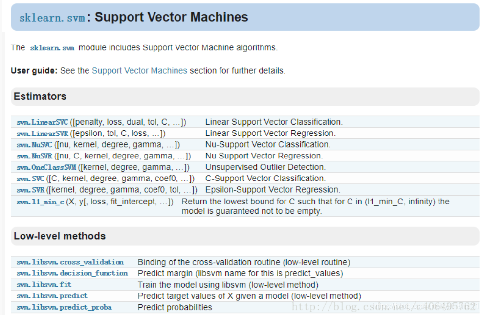
3、SVM支持向量机

SVMs： LinearSVC, Linear SVR, SVC, Nu-SVC, SVR, Nu-SVR, OneClassSVM

from sklearn import svm
from sklearn.svm import SVC
from sklearn.svm import LinearSVC
from sklearn.svm import NuSVC
from sklearn.svm import SVR
from sklearn.svm import LinearSVR

（1）SVM 一对一法

import pandas as pd
import numpy as np
import matplotlib.pyplot as plt
from sklearn import preprocessing
from sklearn.svm import LinearSVC
from sklearn.multiclass import OneVsOneClassifier
from sklearn import model_selection

# Cross validation
X_train, X_test, y_train, y_test = model_selection.train_test_split(X, y, test_size=0.2, random_state=5)
classifier = OneVsOneClassifier(LinearSVC(random_state=0)) #两类样本的分类器
classifier.fit(X_train, y_train)
y_test_pred = classifier.predict(X_test)

# Compute the F1 score of the SVM classifier
f1 = model_selection.cross_val_score(classifier, X, y, scoring='f1_weighted', cv=3) #k折交叉验证
print("F1 score: " + str(round(100*f1.mean(), 2)) + "%")

（2）SVM参数输出

#SVC,基于libsvm，不适用于数量大于10K的数据（时间复杂度高）
#数据准备
data = scio.loadmat("train and test top321.mat") #导入数据
test = data['test'] #待分类数据
testclass = data['testclass']
testclass = np.ravel(testclass)
train = data['train']
trainclass = data['trainclass']
trainclass = np.ravel(trainclass)
#建模分类
clf = SVC(kernel='linear')
clf.fit(train, trainclass)
weight = clf.coef_
print(clf.predict(test))
Pretest = clf.predict(test) #输出分类标签
a = Pretest ^ testclass
acc = (a.size-a.sum())/a.size
print("Accuracy:",acc)
print("支持向量指数:",clf.support_)
print("支持向量",clf.support_vectors_)
print("每一类的支持向量个数",clf.n_support_)
print("支持向量的系数:",clf.dual_coef_)
print("截距:",clf.intercept_)

（3）多分类问题

这块内容不大懂，先放着吧，等后面再梳理下。

SVM解决多分类问题的方法

SVM算法最初是为二值分类问题设计的，当处理多类问题时，就需要构造合适的多类分类器。目前，构造SVM多类分类器的方法主要有两类：一类是直接法，直接在目标函数上进行修改，将多个分类面的参数求解合并到一个最优化问题中，通过求解该最优化问题“一次性”实现多类分类。这种方法看似简单，但其计算复杂度比较高，实现起来比较困难，只适合用于小型问题中；另一类是间接法，主要是通过组合多个二分类器来实现多分类器的构造，常见的方法有one-against-one和one-against-all两种。
a.一对多法（one-versus-rest,简称1-v-r SVMs）。训练时依次把某个类别的样本归为一类,其他剩余的样本归为另一类，这样k个类别的样本就构造出了k个SVM。分类时将未知样本分类为具有最大分类函数值的那类。
b.一对一法（one-versus-one,简称1-v-1 SVMs）。其做法是在任意两类样本之间设计一个SVM，因此k个类别的样本就需要设计k(k-1)/2个SVM。当对一个未知样本进行分类时，最后得票最多的类别即为该未知样本的类别。Libsvm中的多类分类就是根据这个方法实现的。
c.层次支持向量机（H-SVMs）。层次分类法首先将所有类别分成两个子类，再将子类进一步划分成两个次级子类，如此循环，直到得到一个单独的类别为止。

4、数值化转换

对数据进行转换处理。这段代码写的很好。

fit(): Method calculates the parameters μ and σ and saves them as internal objects.
解释：简单来说，就是求得训练集X的均值，方差，最大值，最小值,这些训练集X固有的属性。

transform(): Method using these calculated parameters apply the transformation to a particular dataset.
解释：在fit的基础上，进行标准化，降维，归一化等操作（看具体用的是哪个工具，如PCA，StandardScaler等）。

fit_transform(): joins the fit() and transform() method for transformation of dataset.
解释：fit_transform是fit和transform的组合，既包括了训练又包含了转换。
transform()和fit_transform()二者的功能都是对数据进行某种统一处理（比如标准化~N(0,1)，将数据缩放(映射)到某个固定区间，归一化，正则化等）

label_encoder = []
X_encoded = np.empty(X.shape) #创建0矩阵
for i,item in enumerate(X[0]):
if item.isdigit():
X_encoded[:, i] = X[:, i]
else:
label_encoder.append(preprocessing.LabelEncoder())
X_encoded[:, i] = label_encoder[-1].fit_transform(X[:, i]) #fit_transform既训练又转换。

from sklearn.preprocessing import StandardScaler
sc = StandardScaler()
sc.fit_tranform(X_train) #sc为训练及转换的模型。

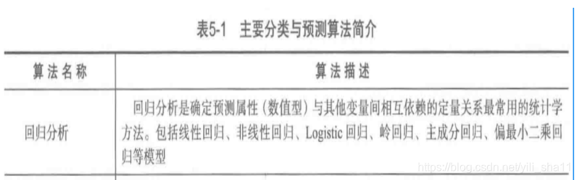
5、变量回归

回归分析是一种预测性的建模技术，它研究的是因变量（目标）和自变量（预测器）之间的关系。这种技术通常用于预测分析，时间序列模型以及发现变量之间的因果关系。例如，司机的鲁莽驾驶与道路交通事故数量之间的关系，最好的研究方法就是回归。
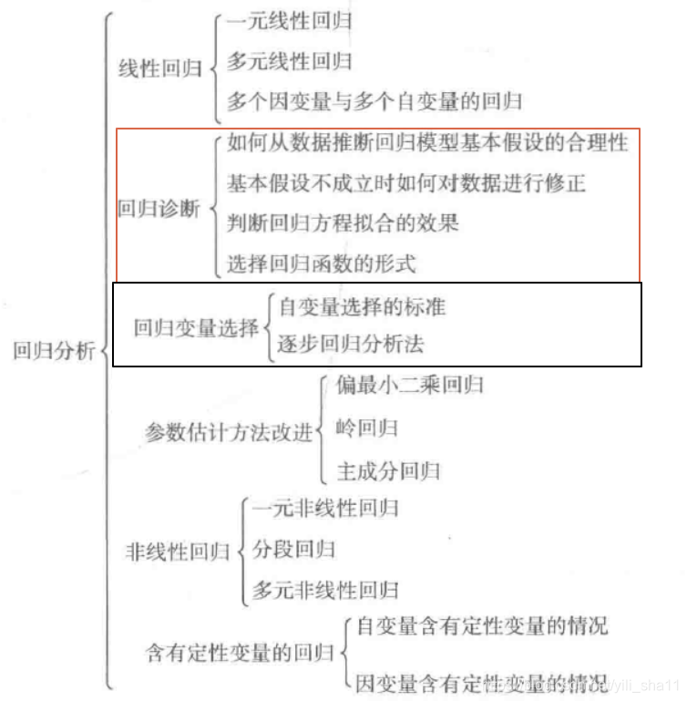
有各种各样的回归技术用于预测。这些技术主要有三个度量（自变量的个数，因变量的类型以及回归线的形状）。

1、各类回归方法导入

（1）单变量/多变量回归、非线性回归

（2）岭回归、主成分回归

2、回归方法导入

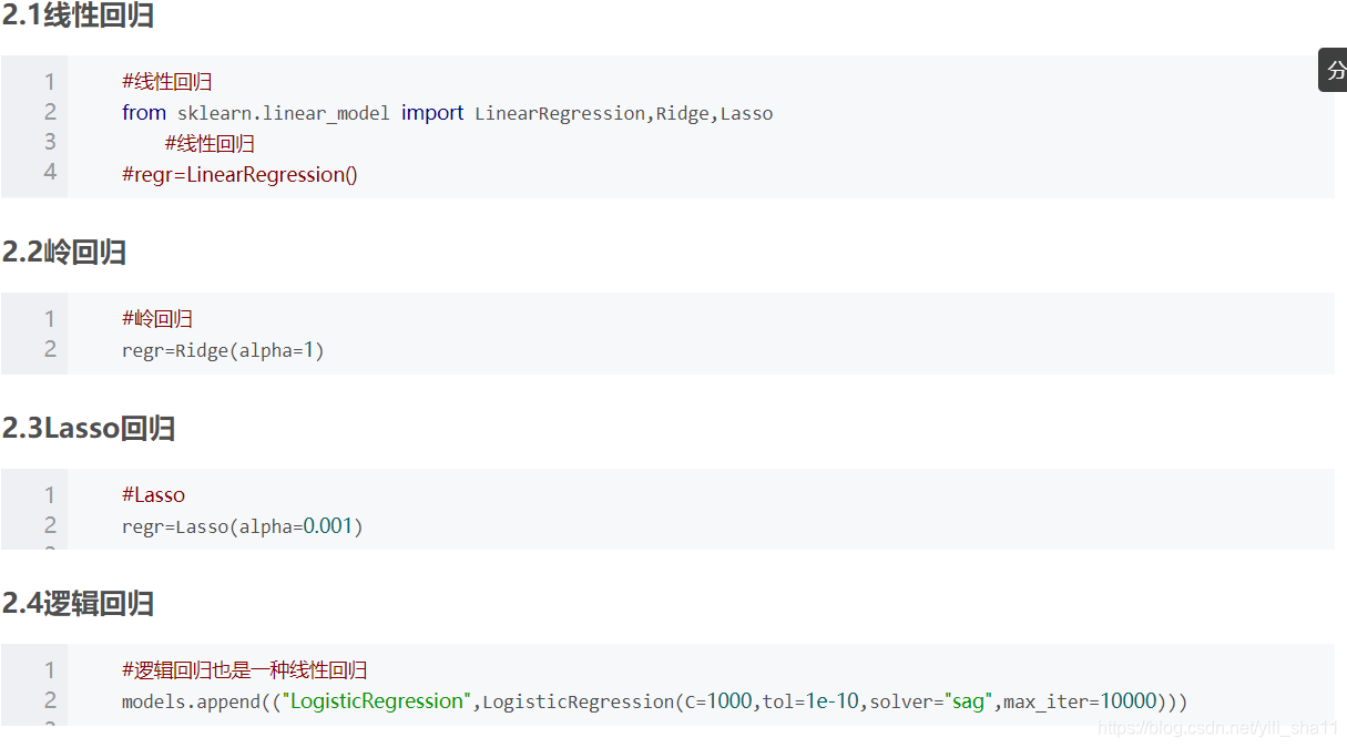
Linear Regression线性回归：线性回归使用最佳的拟合直线（也就是回归线）在因变量（Y）和一个或多个自变量（X）之间建立一种关系。多元线性回归可表示为Y=a+b1X +b2X2+ e，其中a表示截距，b表示直线的斜率，e是误差项。
Logistic Regression逻辑回归：逻辑回归是用来计算“事件=Success”和“事件=Failure”的概率。当因变量的类型属于二元（1 / 0，真/假，是/否）变量时，我们就应该使用逻辑回归。
Polynomial Regression多项式回归：对于一个回归方程，如果自变量的指数大于1，那么它就是多项式回归方程。如下方程所示：y=a+b*x^2 在这种回归技术中，最佳拟合线不是直线。而是一个用于拟合数据点的曲线。
Stepwise Regression逐步回归：在处理多个自变量时，我们可以使用这种形式的回归。在这种技术中，自变量的选择是在一个自动的过程中完成的，其中包括非人为操作。
Ridge Regression岭回归：当数据之间存在多重共线性（自变量高度相关）时，就需要使用岭回归分析。
Lasso Regression套索回归：它类似于岭回归。
ElasticNet回归：ElasticNet是Lasso和Ridge回归技术的混合体。

转载来自：https://www.jianshu.com/p/b476707a7e3c

6、决策树tree

优点：计算复杂度不高，输出结果易于理解，对中间值的缺失值不敏感，可以处理不相关特征数据。
缺点：可能会产生过度匹配的问题。
使用数据类型：数值型和标称型。

学习时，利用训练数据，根据损失函数最小化原则建立决策树模型。预测时，对新的数据，利用决策树模型进行分类。决策树学习通常包括三个步骤：特征选择、决策树的生成以及决策树的修剪。

from sklearn.tree import DecisionTreeClassifier as DTC
dtc = DTC(criterion='entropy') # 建立决策树模型，基于信息熵

#DecisionTreeClassifier(criterion='gini', splitter='best', max_depth=None, min_samples_split=2, min_samples_leaf=1, min_weight_fraction_leaf=0.0, max_features=None, random_state=None, max_leaf_nodes=None, min_impurity_decrease=0.0, min_impurity_split=None, class_weight=None, presort=False)

dtc.fit(x, y) # 训练模型

# 导入相关函数，可视化决策树。
# 导出的结果是一个dot文件，需要安装Graphviz才能将它转换为pdf或png等格式。
from sklearn.tree import export_graphviz
from sklearn.externals.six import StringIO
x = pd.DataFrame(x)
with open("tree.dot", 'w') as f:
f = export_graphviz(dtc, feature_names=x.columns, out_file=f)

（1）ID3算法与cart算法

ID3算法的缺陷

通过对ID3算法进行分析，我们可以知道，ID3算法主要存在以下缺陷：

ID3没有考虑连续型特征，数据集的特征必须是离散型特征
ID3算法采用信息增益大的特征优先建立决策树的结点，但是再计算信息增益的过程中我们发现，在相同条件下，取值比较多的特征比取值少的特征信息增益大
ID3没有对缺失值情况进行处理，现实任务中常会遇到不完整的样本，即样本的某些属性值缺失。
没有考虑过拟合问题

C4.5算法是对ID3算法存在的缺陷进行改进的一种算法，它通过将连续特征离散化来解决ID3算法不能处理离散型数据的问题；通过引入信息增益比来解决信息增益的缺陷；通过增加剪枝操作来解决过拟合的问题。

（2）输出参数

| classes_ : 分类编号
| feature_importances_ : The feature importances. The higher, the more important the feature.
| max_features_ : The inferred value of max_features.
| n_classes_ : The number of classes (for single output problems),
| n_features_ : The number of features when ``fit`` is performed.
| n_outputs_ : The number of outputs when ``fit`` is performed.
| tree_ : Tree object The underlying Tree object.