论文-知识蒸馏

最新推荐文章于 2024-05-15 11:21:13 发布

yywxl

最新推荐文章于 2024-05-15 11:21:13 发布

阅读量2.3k

点赞数 2

分类专栏：深度学习论文 pytorch

本文链接：https://blog.csdn.net/yywxl/article/details/103680152

版权

深度学习同时被 3 个专栏收录

16 篇文章 1 订阅

订阅专栏

论文

13 篇文章 0 订阅

订阅专栏

pytorch

10 篇文章 0 订阅

订阅专栏

文章目录

Structured Knowledge Distillation for Dense Prediction

今天看一篇沈老师他们的工作，是知识蒸馏(knowledge distillation)相关
20200326 今天再看一遍这个文章，以前没有关注他的pair-wise distillation,今天要做相关工作，重新看一遍，复现相关代码2333

github传送

Structured Knowledge Distillation for Dense Prediction

Previous knowledge distillation strategies used for dense prediction tasks often directly borrow the distillation scheme for image classification and perform knowledge distillation for each pixel separately, leading to sub-optimal performance

文章摘要说，以前的KD都是对每一个像素学习知识，会得到一个次优的解。他说的是对于dense prediction。这是为什么呢？

Here we propose to distill structured knowledge from large networks to small networks, taking into account the fact that dense prediction is a structured prediction problem.

由于dense prediction就是一个结构预测的问题，所以提出了一个‘蒸馏结构知识’的方法。有两种结构蒸馏方案,他管以前的KD叫做pixel-wise distillation

pair-wise distillation

The pair-wise distillation scheme is motivated by the widely-studied pair-wise Markov random field framework. 引文23

holistic distillation

The holistic distillation scheme aims to align higher-order consistencies

Specifically, we study two structured distillation schemes:
i) pair-wise distillation that distills the pairwise similarities by building a static graph;
and ii) holistic distillation that uses adversarial training to distill holistic knowledge.

Dense Prediction

Dense prediction is a category of fundamental problems in computer vision, which learns a mapping from input objects to complex output structures, including semantic segmentation, depth estimation and object detection, among many others.

将输入映射为复杂的结构输出，那么他的这种结构蒸馏好像不是我们图像恢复需要的？(思想好像可以照搬，但是他的设计可能更关注dense structure)

基于以上考虑，看了下pipeline
SKD
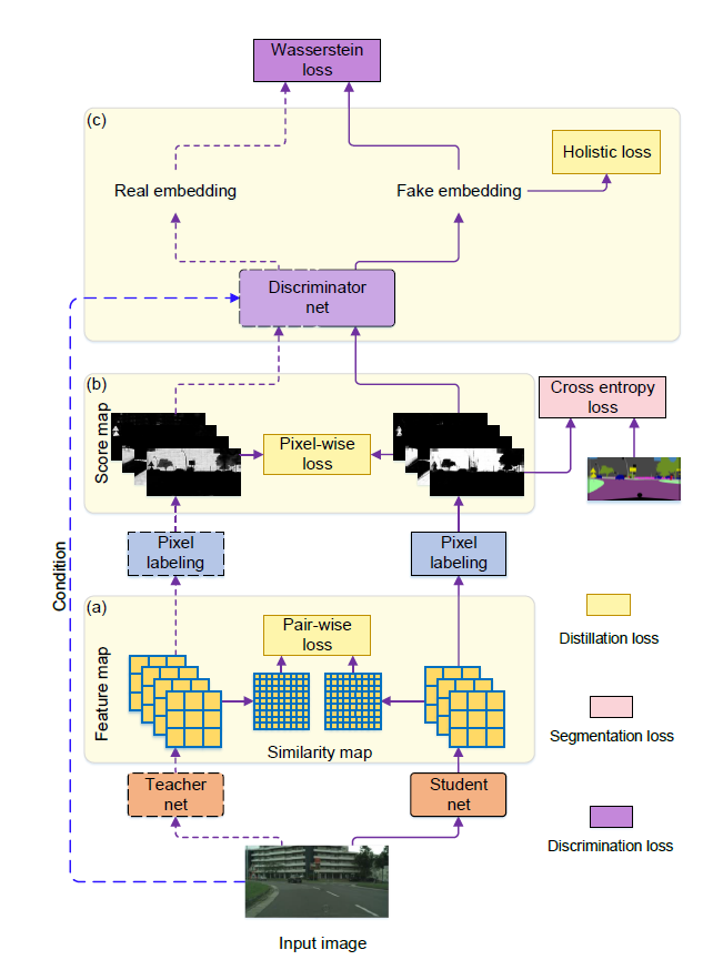
除了holistic loss不清楚怎么算的，其他好像很有道理。

好像文章都很热衷于各种trick疯狂刷指标。。。。
文章将他应用在语义分割，深度估计，目标检测

方法
I $W\times H\times 3$ RGB输入
F $W\times H\times N$ 输入I的feature map
Q $W\times H\times C$ F经过a classifier计算的分割map？？？上采样到 $W\times H$ 作为分割结果。
Segmentation Q feature map变换后的结果作为分割即分类的结果
？这个变换是什么？

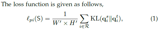
Pixel-wise distillation
计算S和T输出的概率图之间KL散度

Pair-wise distillation
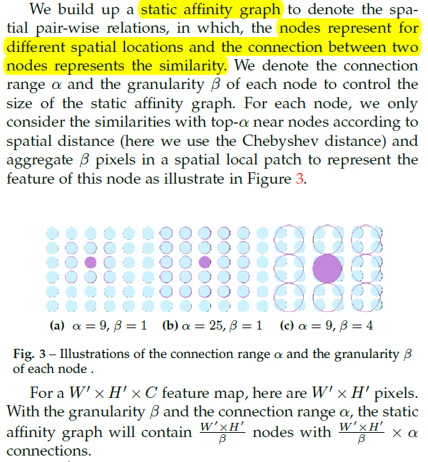
static affinity graph表示空间成对的关系

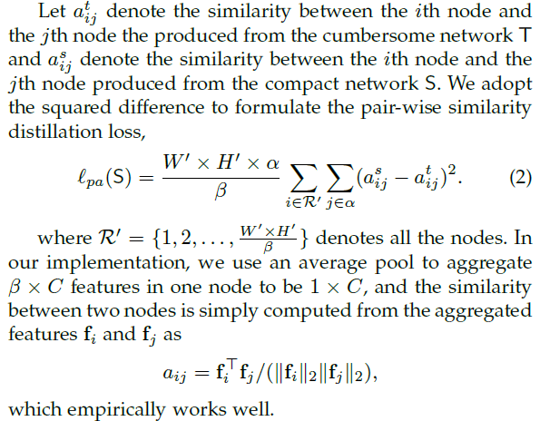
$\beta$ 使用平均池化得到聚合的节点

翻译一下：

节点(Node)表示不同的空间位置，两个节点之间的连接表示相似性(similarity)
每个节点的连接范围（connection range alpha）和间隔尺寸(granularity beta)控制着静态关联图(static affinity graph)的大小
由上面图示可知，alpha表示相邻的节点，beta表示聚合多少个像素作为一个节点
总共会有 $\frac{W'\times H'}{\beta}$ 个节点，S、T网络的静态关联图的L2 Loss就是pair-wise KD
这里还是有点不太清楚，每个node之间的相似性 $a_{ij}$ 就是余弦距离，但是 $\alpha$ 起到什么作用，因为这样会生成NodexNode个大小的SAG
看代码

class CriterionPairWiseforWholeFeatAfterPool(nn.Module):
    def __init__(self, scale, feat_ind):
        '''inter pair-wise loss from inter feature maps'''
        super(CriterionPairWiseforWholeFeatAfterPool, self).__init__()
        self.criterion = sim_dis_compute
        self.feat_ind = feat_ind #-5
        self.scale = scale #0.5

    def forward(self, preds_S, preds_T):
        '''
        :preds_S 学生网络feature
        :preds_T 教师网络feature
        '''
        feat_S = preds_S[self.feat_ind]
        feat_T = preds_T[self.feat_ind]
        #这里注意detach的写法,好像补写也ok？
        feat_T.detach()

        total_w, total_h = feat_T.shape[2], feat_T.shape[3]
        #patch_w, patch_h scale即beta聚合后feature大小，按照文章说法不是avgpooling，然后余弦距离
        #这里scale还不是我想的将featurescale的大小，而是pool的大小，即beta aggregate后feature大小为 int(1/scale)-(2)
        #这么小吗，一个feature只只剩下1/scale x 1/scale (4)个node，那alpha有什么用。。。
        patch_w, patch_h = int(total_w*self.scale), int(total_h*self.scale)
        #maxpooling ceil_mode 是否将kernel以外不满足大小的部分也做maxpooling，False则舍弃
        maxpool = nn.MaxPool2d(kernel_size=(patch_w, patch_h), stride=(patch_w, patch_h), padding=0, ceil_mode=True) # change
        loss = self.criterion(maxpool(feat_S), maxpool(feat_T))
        return loss
def L2(f_):
    '''
    按通道求根号下(求和(x))
    -> c通道二范数
    '''
    return (((f_**2).sum(dim=1))**0.5).reshape(f_.shape[0],1,f_.shape[2],f_.shape[3]) + 1e-8

def similarity(feat):
    '''
    计算相似性
    :feat feature map after pooling
    -> nodexnode similarity matrix
    '''
    feat = feat.float()
    tmp = L2(feat).detach()
    #先除以范数归一化
    feat = feat/tmp
    #reshape -> nxcxhw
    feat = feat.reshape(feat.shape[0],feat.shape[1],-1)
    #底下这个爱因斯坦求和是真的秀，由于node数量只有4ge，分patch都省了，直接矩阵相乘即可
    #这样返回nodexnode的similarity feature,node所在通道和其他所有node通道之间的向量点积
    return torch.einsum('icm,icn->imn', [feat, feat])

def sim_dis_compute(f_S, f_T):
    '''
    :f_S, f_T pooling后的feature
    '''
    sim_err = ((similarity(f_T) - similarity(f_S))**2)/((f_T.shape[-1]*f_T.shape[-2])**2)/f_T.shape[0]
    sim_dis = sim_err.sum()
    return sim_dis

除了对于beta aggregate 意外，pair-wise 好像没有什么疑问
后面实验部分对于这个刚好有讨论

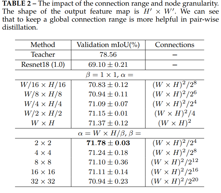
文章实验好像和代码不一样啊？认为beta=2 alpha=global是语义分割效果最好，并且在alpha和beta之间优先增大beta的值减小计算量
按照文章的实验改一下代码写一个pair-wise kd loss
文章还对比了三种知识蒸馏的方法，mark待看

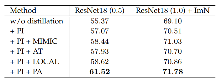
斗胆猜测一下上面三种算法的做法

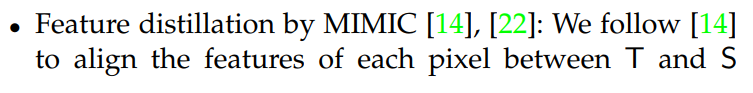
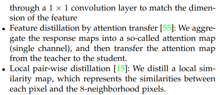
用1x1卷积匹配维度，在计算pixel-wise kd
attention 计算T的feature的attention map(怎样计算不可知)，然后衡量attention map之间度量
这文章略相似，多了beta 聚合和alpha global 连接

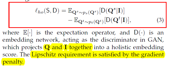
Holistic distillation
使用全局蒸馏时，使用了conditional GAN，由于离散的JS散度(两个分布相差过大，KL没意义，JS是常数)，使用Wasserstein distance or Earth Mover distance

Discriminator使用self-attention residual block,self-attention和residual block的位置和数量见论文
以上，很多概念都不是特别懂
conditional GAN
将输出和条件(输入图像)concatenate送到net_D
Wasserstein distance
wgan 限制w范围的一个参考写法

for p in discriminator.parameters():
    p.data.clamp_(-opt.clip_value, opt.clip_value)

$Q^{s}$ 和 $Q^{t}$ 是怎么embedding的
Discriminator 最后输出是什么，概率吗？
fully convolutional neural network全卷积网络

We further add a pooling layer to pool the holistic embedding into a score
pooling as score

The Lipschitz requirement is satisfied by the gradient penalty
这个怎么写？

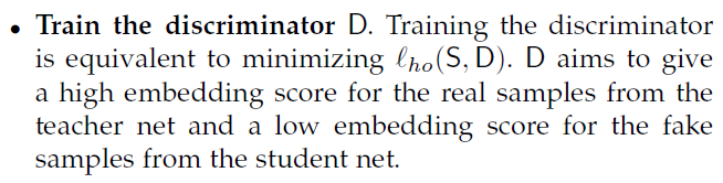
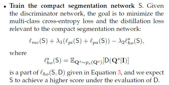
Optimization

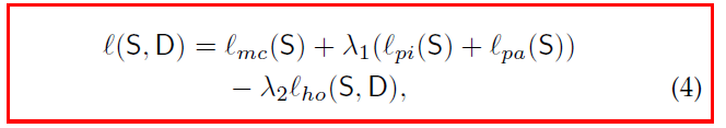
$\lambda_{2}$ 前为负号？(对于生成网络似乎是这样)

lambda1=10, lambda2=0.1

以上大概是文章的介绍部分，有很多地方还不是很清楚，开始读代码。。。。

self-attention模块
具体原理待看，可以参考这个博客,其实还是不懂，因为对RNN不太理解,代码来看就是下面这个过程，先跑起来，然后再看，MARK

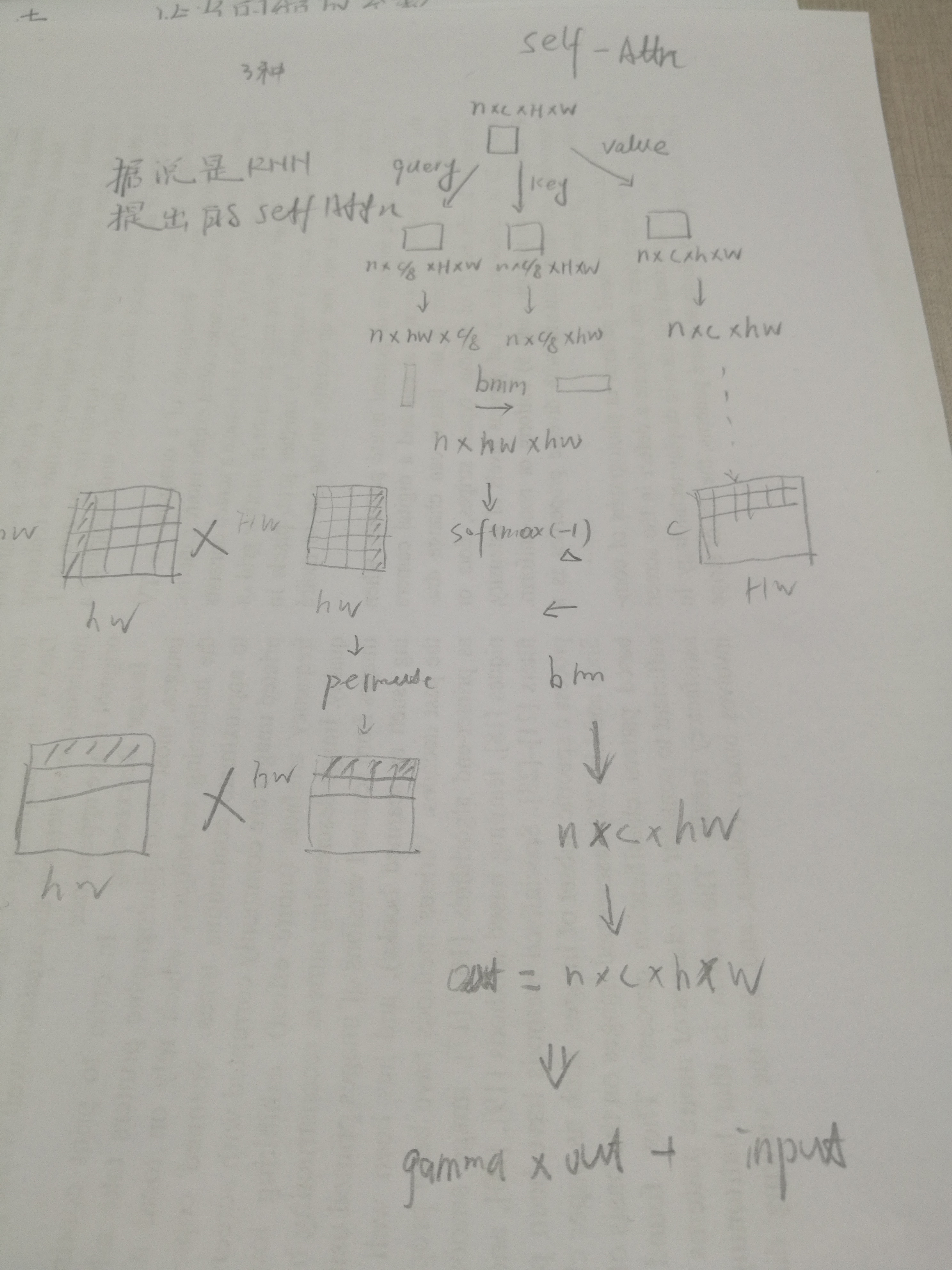
~~这个辣鸡图softmax那里画错了，就不要看了~~
对于原理我不能理解，但是看代码可以连接他的模块
proj_query
proj_key
proj_value
以上三个都是卷积得到的投影，key-value, query计算和key的相似度，作为权值乘以value

class selfAttn(nn.Module):
    def __init__(self, dim):
        super(selfAttn, self).__init__()
        self.query_conv = nn.Conv2d(dim, dim//8, 1)
        self.key_conv = nn.Conv2d(dim, dim//8, 1)
        self.value_conv = nn.Conv2d(dim, dim, 1)
        self.gamma = nn.Parameter(torch.zeros(1))
        self.softmax = nn.Softmax(dim=-1)
        #这里dim=-1其实是每一行的所有列进行softmax, 所以归一化表现在每一行上
        #即每一行的sum=1
    def forward(self, x):
        n, c, h, w = x.shape
        proj_query = self.query_conv(x).view(n, -1, h*w).permute(0, 2, 1) #nxc'xhw -> nxhwxc'
        proj_key = self.key_conv(x).view(n, -1, h*w) #nxc'xhw
        #计算相似度
        energy = torch.bmm(proj_query, proj_key) #nxwhxwh
        attention = self.softmax(energy)
        proj_value = self.value_conv(x).view(n, -1, h*w) #nxcxhw
        
        out = torch.bmm(proj_value, attention.permute(0, 2, 1)) #nxcxhw,
        print(out.shape)
        out = out.view(n, c, h, w)
        out = self.gamma*out + x #resnet skip connection
        print(proj_query.shape, proj_key.shape, energy.shape, attention.shape, proj_key.shape)
        return out, attention

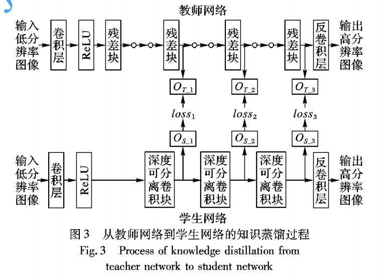
基于知识蒸馏的超分辨率卷积神经网络压缩方法

上面的文章和这篇文章都是知其然而不知其所以然

motivation

他有一篇引文说不同层次的特征图代表不同的信息，且传递中间的feature会比输出更有效，所以它采用的以下方法，使用三个层次的信息
网络结构

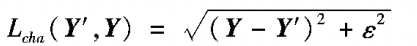
loss函数

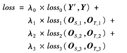
以上超参 0 = 1+2+3,1:1就好

training

特征图统计

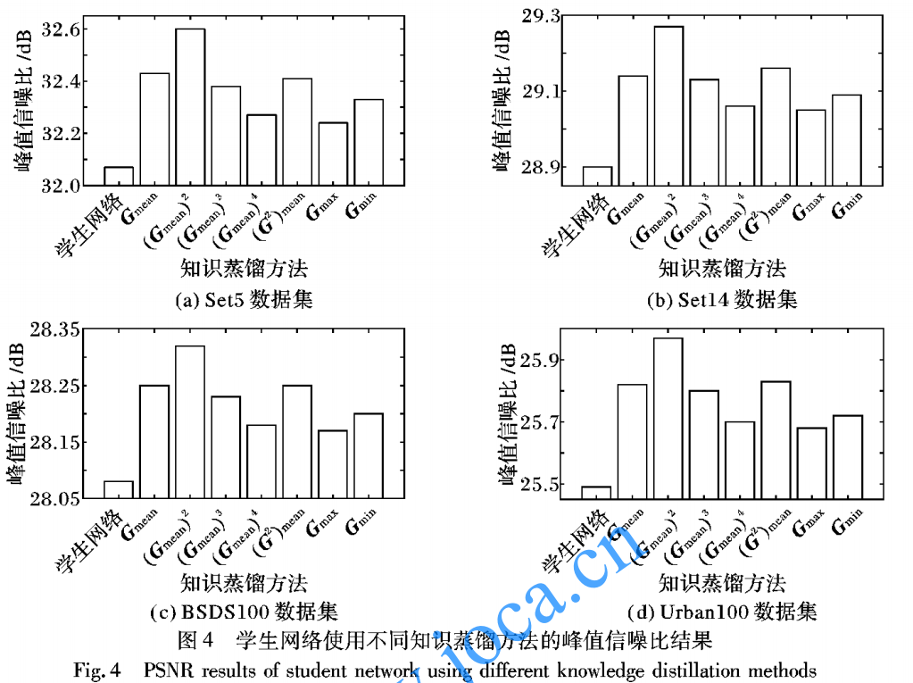
结论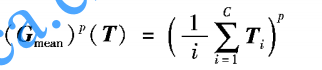：，这个统计量最优

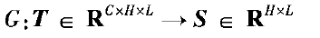
从上面来看这个应该是按通道的特征统计
teacher网络的大小
teacher网络越大越好，但是过大以后提升越来越小

Lightweight Image Super-Resolution with Information Multi-distillation Network

都找不到low-level知识蒸馏的文章，在github awesome-knowledge-distillation项目中只找到一篇超分相关的，还是西电的2333，看一下吧

recently, Zhang et al. also introduced spatial attention (non-local module) into the residual block and then constructed residual non-local attention network (RNAN) [37] for various image restoration tasks.

spatial attention for various image restoration tasks ——可以关注下

文章想要解决计算量的问题从

参数量 parameters
depth
resolution
方面进行设计
文章受启发与IDN提出了IMDN(infomation multi-distillation network)
,构建了IMDB(blocks)提取信息包括两部分，一部分retains partial information，一部分feature treats other features,
aggregating features distilled这个就叫做蒸馏？
他使用了contrast-aware channel attention layer, specifically related to the low-level vision task,他说这种和低级的视觉任务很相关，关注！

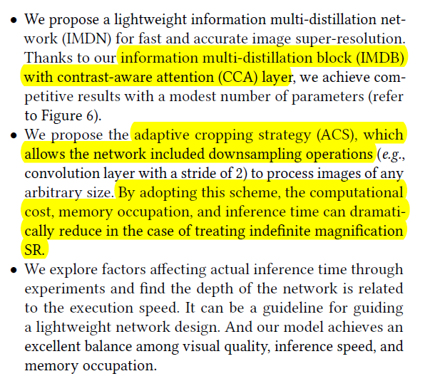
文章的contributions，最后一个是认真的？网络的深度和推断速度相关…可能我理解的错了，看他的实验吧
paper

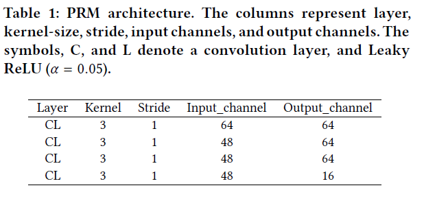
网络框架

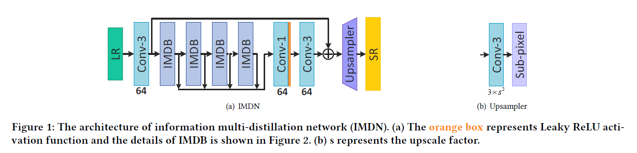
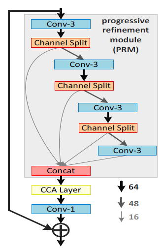
上面依次是网络主体IMDN，上采样UP，信息多蒸馏块IMDB，对比度感知通道注意层CCA
疑问：1. channel split？就是将channel分为两部分(64=16+48),前面的层表示refined features
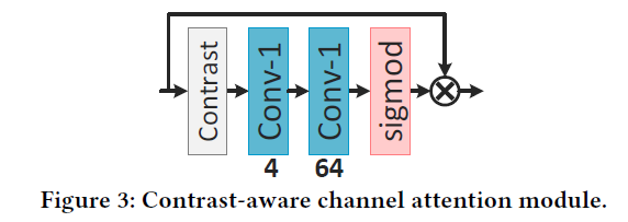
2. contrast？

在这里插入图片描述
回答上面疑问2：
CCA
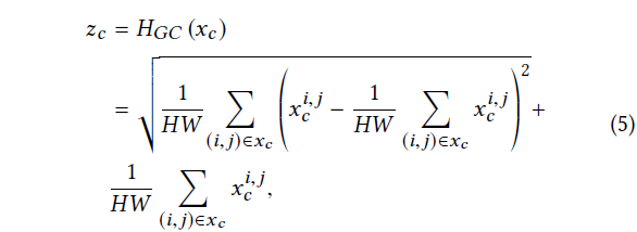
CCA做了上面这样一件事，按channel统计均值和方差作为attention相加，总感觉这样的加法或者乘法没有什么道理，并不能说服我，但是他是网络学习出来的特征，可能代表一些东西。上面公式计算出来的结果是 $c\times1\times1$ ?

Adaptive cropping stategy ACS-IMDN_AS
他的思想就是将图像裁成四块并行计算，允许一份的重叠，计算完成后再舍弃重叠部分拼接
他这是任意尺寸的图像放大固定倍数，而不是任意倍数的超分。。。。失望

好，到这里我们大概了解了知识蒸馏的做法，人们将他归为transfer learning迁移学习，就是将大网络的先验知识传送给小网络，那么这样做为什么可行呢？？然我们从头开始学习**Knowlledge Distillation**

yywxl

关注

2
点赞
踩
6

收藏

觉得还不错? 一键收藏
1
评论
论文-知识蒸馏

今天看一篇沈老师他们的工作，是知识蒸馏(knowledge distillation)相关github传送Structured Knowledge Distillation for Dense PredictionPrevious knowledge distillation strategies used for dense prediction tasks often direct...
复制链接

扫一扫