


基于空间注意力机制SAM的GoogLeNet实现人脸关键点检测并自动添加表情贴纸
使用神经网路实现人脸关键点检测,并根据人脸关键点添加表情贴纸已广泛应用于直播、短视频、特效相机、视频社交等泛娱乐场景中,为用户提供了美颜、滤镜、贴纸等多种特效。
本文在TC.Long老师的项目(使用resnet50作为backbone)的基础上做改进,使用GoogLeNet加BN层加速模型收敛,使用空间注意力机制提高模型效果。
参考资料:
- 飞桨深度学习学院——「高层API深度学习7日打卡营」
- 飞桨『高层API助你快速上手深度学习』之人脸关键点检测
- 一文搞懂卷积网络之一(【动态图】从LeNet到GoogLeNet)
- 新年美食鉴赏——基于注意力机制CBAM的美食101分类
- Hub人脸关键点检测实现耳朵和鼻子贴纸
一、效果展示
人脸关键点检测,是输入一张人脸图片,模型会返回人脸关键点的一系列坐标,从而定位到人脸的关键信息。最后再根据人脸关键点将表情贴纸添加到人脸上。

二、数据准备
1.解压数据集
本项目所采用的数据集来源为github的开源项目
目前该数据集已上传到 AI Studio 人脸关键点识别,加载后可以直接使用下面的命令解压。
!unzip data/data69065/data.zip
解压后的数据集结构为
data/
|—— test
|   |—— Abdel_Aziz_Al-Hakim_00.jpg
    ... ...
|—— test_frames_keypoints.csv
|—— training
|   |—— Abdullah_Gul_10.jpg
    ... ...
|—— training_frames_keypoints.csv
其中,training 和 test 文件夹分别存放训练集和测试集。training_frames_keypoints.csv 和 test_frames_keypoints.csv 存放着训练集和测试集的标签。接下来,我们先来观察一下 training_frames_keypoints.csv 文件,看一下训练集的标签是如何定义的。
2.数据集介绍
key_pts_frame = pd.read_csv('data/training_frames_keypoints.csv') # 读取数据集
print('Number of images: ', key_pts_frame.shape[0]) # 输出数据集大小
key_pts_frame.head(5) # 看前五条数据
Number of images: 3462
| Unnamed: 0 | 0 | 1 | 2 | 3 | 4 | 5 | 6 | 7 | 8 | ... | 126 | 127 | 128 | 129 | 130 | 131 | 132 | 133 | 134 | 135 | |
|---|---|---|---|---|---|---|---|---|---|---|---|---|---|---|---|---|---|---|---|---|---|
| 0 | Luis_Fonsi_21.jpg | 45.0 | 98.0 | 47.0 | 106.0 | 49.0 | 110.0 | 53.0 | 119.0 | 56.0 | ... | 83.0 | 119.0 | 90.0 | 117.0 | 83.0 | 119.0 | 81.0 | 122.0 | 77.0 | 122.0 |
| 1 | Lincoln_Chafee_52.jpg | 41.0 | 83.0 | 43.0 | 91.0 | 45.0 | 100.0 | 47.0 | 108.0 | 51.0 | ... | 85.0 | 122.0 | 94.0 | 120.0 | 85.0 | 122.0 | 83.0 | 122.0 | 79.0 | 122.0 |
| 2 | Valerie_Harper_30.jpg | 56.0 | 69.0 | 56.0 | 77.0 | 56.0 | 86.0 | 56.0 | 94.0 | 58.0 | ... | 79.0 | 105.0 | 86.0 | 108.0 | 77.0 | 105.0 | 75.0 | 105.0 | 73.0 | 105.0 |
| 3 | Angelo_Reyes_22.jpg | 61.0 | 80.0 | 58.0 | 95.0 | 58.0 | 108.0 | 58.0 | 120.0 | 58.0 | ... | 98.0 | 136.0 | 107.0 | 139.0 | 95.0 | 139.0 | 91.0 | 139.0 | 85.0 | 136.0 |
| 4 | Kristen_Breitweiser_11.jpg | 58.0 | 94.0 | 58.0 | 104.0 | 60.0 | 113.0 | 62.0 | 121.0 | 67.0 | ... | 92.0 | 117.0 | 103.0 | 118.0 | 92.0 | 120.0 | 88.0 | 122.0 | 84.0 | 122.0 |
5 rows × 137 columns
上表中每一行都代表一条数据,其中,第一列是图片的文件名,之后从第0列到第135列,就是该图的关键点信息。因为每个关键点可以用两个坐标表示,所以 136/2 = 68,就可以看出这个数据集为68点人脸关键点数据集。
目前常用的人脸关键点标注,有如下点数的标注:
- 5点
- 21点
- 68点
- 98点
本次数据集采用68点标注,标注顺序如下:
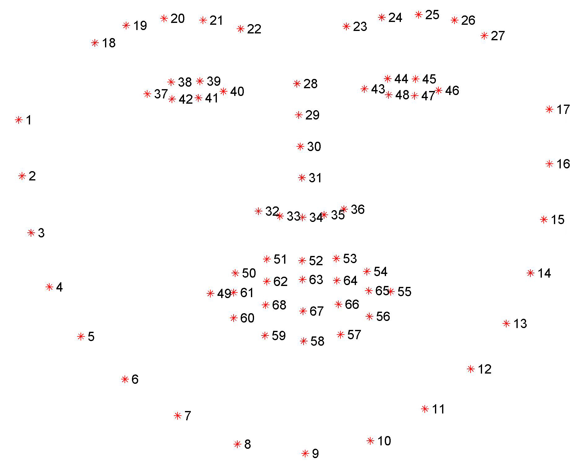
- 1-17:人脸的下轮廓
- 18-27:眉毛
- 28-36: 鼻子
- 37-48:眼睛
- 49-68:嘴巴
# 计算标签的均值和标准差,用于标签的归一化
key_pts_values = key_pts_frame.values[:,1:] # 取出标签信息
data_mean = key_pts_values.mean() # 计算均值
data_std = key_pts_values.std()   # 计算标准差
print('标签的均值为:', data_mean)
print('标签的标准差为:', data_std)
标签的均值为: 104.4724870017331
标签的标准差为: 43.17302271754281
查看图像
def show_keypoints(image, key_pts):
    """
    Args:
        image: 图像信息
        key_pts: 关键点信息,
    展示图片和关键点信息
    """
    plt.imshow(image.astype('uint8'))  # 展示图片信息
    for i in range(len(key_pts)//2,):
        plt.scatter(key_pts[i*2], key_pts[i*2+1], s=20, marker='.', c='b') # 展示关键点信息
# 展示单条数据
n = 421 # n为数据在表格中的索引
image_name = key_pts_frame.iloc[n, 0] # 获取图像名称
key_pts = key_pts_frame.iloc[n, 1:].as_matrix() # 将图像label格式转为numpy.array的格式
key_pts = key_pts.astype('float').reshape(-1) # 获取图像关键点信息
print(key_pts.shape)
plt.figure(figsize=(5, 5)) # 展示的图像大小
show_keypoints(mpimg.imread(os.path.join('data/training/', image_name)), key_pts) # 展示图像与关键点信息
plt.show() # 展示图像
(136,)

3.数据集定义
使用飞桨框架高层API的 paddle.io.Dataset 自定义数据集类,具体可以参考官网文档 自定义数据集。
# 按照Dataset的使用规范,构建人脸关键点数据集
from paddle.io import Dataset

class FacialKeypointsDataset(Dataset):
    # 人脸关键点数据集
    """
    步骤一:继承paddle.io.Dataset类
    """
    def __init__(self, csv_file, root_dir, transform=None):
        """
        步骤二:实现构造函数,定义数据集大小
        Args:
            csv_file (string): 带标注的csv文件路径
            root_dir (string): 图片存储的文件夹路径
            transform (callable, optional): 应用于图像上的数据处理方法
        """
        self.key_pts_frame = pd.read_csv(csv_file) # 读取csv文件
        self.root_dir = root_dir # 获取图片文件夹路径
        self.transform = transform # 获取 transform 方法

    def __getitem__(self, idx):
        """
        步骤三:实现__getitem__方法,定义指定index时如何获取数据,并返回单条数据(训练数据,对应的标签)
        """

        image_name = os.path.join(self.root_dir,
                                self.key_pts_frame.iloc[idx, 0])
        # 获取图像
        image = mpimg.imread(image_name)

        # 图像格式处理,如果包含 alpha 通道,那么忽略它
        if(image.shape[2] == 4):
            image = image[:,:,0:3]

        # 获取关键点信息
        key_pts = self.key_pts_frame.iloc[idx, 1:].as_matrix()
        key_pts = key_pts.astype('float').reshape(-1) # [136, 1]

        # 如果定义了 transform 方法,使用 transform方法
        if self.transform:
            image, key_pts = self.transform([image, key_pts])

        # 转为 numpy 的数据格式
        image = np.array(image, dtype='float32')
        key_pts = np.array(key_pts, dtype='float32')

        return image, key_pts

    def __len__(self):
        """
        步骤四:实现__len__方法,返回数据集总数目
        """
        return len(self.key_pts_frame) # 返回数据集大小,即图片的数量
4.训练集可视化
实例化数据集并显示一些图像
# 构建一个数据集类
face_dataset = FacialKeypointsDataset(csv_file='data/training_frames_keypoints.csv',
                                      root_dir='data/training/')

# 输出数据集大小
print('数据集大小为: ', len(face_dataset))
# 根据 face_dataset 可视化数据集
num_to_display = 5

for i in range(num_to_display):

    # 定义图片大小
    fig = plt.figure(figsize=(20,10))

    # 随机选择图片
    rand_i = np.random.randint(0, len(face_dataset))
    sample = face_dataset[rand_i]

    # 输出图片大小和关键点的数量
    print(i, sample[0].shape, sample[1].shape)

    # 设置图片打印信息
    ax = plt.subplot(1, num_to_display, i + 1)
    ax.set_title('Sample #{}'.format(i))

    # 输出图片
    show_keypoints(sample[0], sample[1])
数据集大小为:  3462
0 (180, 164, 3) (136,)
1 (274, 288, 3) (136,)
2 (172, 169, 3) (136,)
3 (177, 154, 3) (136,)
4 (258, 243, 3) (136,)


上述代码虽然完成了数据集的定义,但是还有一些问题,如:
- 每张图像的大小不一样,图像大小需要统一以适配网络输入要求
- 图像格式需要适配模型的格式输入要求
- 数据量比较小,没有进行数据增强
这些问题都会影响模型最终的性能,所以需要对数据进行预处理。
5.图像预处理
对图像进行预处理,包括灰度化、归一化、重新设置尺寸、随机裁剪,修改通道格式等等,以满足数据要求;每一类的功能如下:
- 灰度化:丢弃颜色信息,保留图像边缘信息;识别算法对于颜色的依赖性不强,加上颜色后鲁棒性会下降,而且灰度化图像维度下降(3->1),保留梯度的同时会加快计算。
- 归一化:加快收敛
- 重新设置尺寸:数据增强
- 随机裁剪:数据增强
- 修改通道格式:改为模型需要的结构
# 标准化自定义 transform 方法
class TransformAPI(object):
    """
    步骤一:继承 object 类
    """
    def __call__(self, data):
        """
        步骤二:在 __call__ 中定义数据处理方法
        """

        processed_data = data
        return  processed_data
import paddle.vision.transforms.functional as F

class GrayNormalize(object):
    # 将图片变为灰度图,并将其值放缩到[0, 1]
    # 将 label 放缩到 [-1, 1] 之间

    def __call__(self, data):
        image = data[0]   # 获取图片
        key_pts = data[1] # 获取标签

        image_copy = np.copy(image)
        key_pts_copy = np.copy(key_pts)

        # 灰度化图片
        gray_scale = paddle.vision.transforms.Grayscale(num_output_channels=3)
        image_copy = gray_scale(image_copy)

        # 将图片值放缩到 [0, 1]
        image_copy = image_copy / 255.0

        # 将坐标点放缩到 [-1, 1]
        mean = data_mean # 获取标签均值
        std = data_std   # 获取标签标准差
        key_pts_copy = (key_pts_copy - mean)/std

        return image_copy, key_pts_copy

class Resize(object):
    # 将输入图像调整为指定大小

    def __init__(self, output_size):
        assert isinstance(output_size, (int, tuple))
        self.output_size = output_size

    def __call__(self, data):

        image = data[0]    # 获取图片
        key_pts = data[1]  # 获取标签

        image_copy = np.copy(image)
        key_pts_copy = np.copy(key_pts)

        h, w = image_copy.shape[:2]
        if isinstance(self.output_size, int):
            if h > w:
                new_h, new_w = self.output_size * h / w, self.output_size
            else:
                new_h, new_w = self.output_size, self.output_size * w / h
        else:
            new_h, new_w = self.output_size

        new_h, new_w = int(new_h), int(new_w)

        img = F.resize(image_copy, (new_h, new_w))

        # scale the pts, too
        key_pts_copy[::2] = key_pts_copy[::2] * new_w / w
        key_pts_copy[1::2] = key_pts_copy[1::2] * new_h / h

        return img, key_pts_copy


class RandomCrop(object):
    # 随机位置裁剪输入的图像

    def __init__(self, output_size):
        assert isinstance(output_size, (int, tuple))
        if isinstance(output_size, int):
            self.output_size = (output_size, output_size)
        else:
            assert len(output_size) == 2
            self.output_size = output_size

    def __call__(self, data):
        image = data[0]
        key_pts = data[1]

        image_copy = np.copy(image)
        key_pts_copy = np.copy(key_pts)

        h, w = image_copy.shape[:2]
        new_h, new_w = self.output_size

        top = np.random.randint(0, h - new_h)
        left = np.random.randint(0, w - new_w)

        image_copy = image_copy[top: top + new_h,
                      left: left + new_w]

        key_pts_copy[::2] = key_pts_copy[::2] - left
        key_pts_copy[1::2] = key_pts_copy[1::2] - top

        return image_copy, key_pts_copy

class ToCHW(object):
    # 将图像的格式由HWC改为CHW
    def __call__(self, data):

        image = data[0]
        key_pts = data[1]

        transpose = T.Transpose((2, 0, 1)) # 改为CHW
        image = transpose(image)

        return image, key_pts
看一下每种图像预处理方法的的效果。
import paddle.vision.transforms as T

# 测试 Resize
resize = Resize(256)

# 测试 RandomCrop
random_crop = RandomCrop(128)

# 测试 GrayNormalize
norm = GrayNormalize()

# 测试 Resize + RandomCrop,图像大小变到250*250, 然后截取出224*224的图像块
composed = paddle.vision.transforms.Compose([Resize(250), RandomCrop(224)])

test_num = 666 # 测试的数据下标
data = face_dataset[test_num]

transforms = {'None': None,
              'norm': norm,
              'random_crop': random_crop,
              'resize': resize ,
              'composed': composed}
for i, func_name in enumerate(['None', 'norm', 'random_crop', 'resize', 'composed']):

    # 定义图片大小
    fig = plt.figure(figsize=(20,10))

    # 处理图片
    if transforms[func_name] != None:
        transformed_sample = transforms[func_name](data)
    else:
        transformed_sample = data

    # 设置图片打印信息
    ax = plt.subplot(1, 5, i + 1)
    ax.set_title(' Transform is #{}'.format(func_name))

    # 输出图片
    show_keypoints(transformed_sample[0], transformed_sample[1])


图像归一化后,肉眼看上去是黑色的,这是因为像素值由0-255缩放到了0-1,越趋近于0越黑,越趋近于255越白,所以归一化后的图像看上去是黑的
6.使用数据预处理的方式完成数据定义
让我们将 Resize、RandomCrop、GrayNormalize、ToCHW 应用于新的数据集
from paddle.vision.transforms import Compose

data_transform = Compose([Resize(256), RandomCrop(224), GrayNormalize(), ToCHW()])

# create the transformed dataset
train_dataset = FacialKeypointsDataset(csv_file='data/training_frames_keypoints.csv',
                                       root_dir='data/training/',
                                       transform=data_transform)
print('Number of train dataset images: ', len(train_dataset))

for i in range(4):
    sample = train_dataset[i]
    print(i, sample[0].shape, sample[1].shape)

test_dataset = FacialKeypointsDataset(csv_file='data/test_frames_keypoints.csv',
                                             root_dir='data/test/',
                                             transform=data_transform)

print('Number of test dataset images: ', len(test_dataset))
Number of train dataset images:  3462
0 (3, 224, 224) (136,)
1 (3, 224, 224) (136,)
2 (3, 224, 224) (136,)
3 (3, 224, 224) (136,)
Number of test dataset images:  770
三、模型组网
1.网络介绍
分类任务中,有多少个类别,输出维度就是多少。不同的是,人脸关键点检测任务中,输出为 人脸关键点的数量*2,即每个人脸关键点的横坐标与纵坐标,这样就可以完成人脸关键点检测任务了。
-
Inception模块

-
空间注意力模块

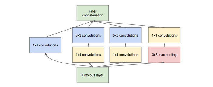
2.Inception模块
GoogLeNet是由Inception模块进行组成的,GoogLeNet采用了模块化的结构,因此修改网络结构时非常简单方便。
import paddle
import paddle.nn as nn

# GoogLeNet加BN层加速模型收敛
class Inception(nn.Layer): # 定义Inception块(Inception v1)
    def __init__(self,c1, c2, c3, c4):
        super(Inception, self).__init__()

        self.relu = nn.ReLU()
        self.p1_1 = nn.Conv2D(c1[0], c1[1], 1)
        self.p2_1 = nn.Conv2D(c1[0], c2[0], 1)
        self.p2_2 = nn.Conv2D(c2[0], c2[1], 3, padding=1)
        self.p3_1 = nn.Conv2D(c1[0], c3[0], 1)
        self.p3_2 = nn.Conv2D(c3[0], c3[1], 5, padding=2)
        self.p4_1 = nn.MaxPool2D(kernel_size=3, stride=1, padding=1)
        self.p4_2 = nn.Conv2D(c1[0], c4, 1)

    def forward(self, x):
        p1 = self.relu(self.p1_1(x))
        p2 = self.relu(self.p2_2(self.p2_1(x)))
        p3 = self.relu(self.p3_2(self.p3_1(x)))
        p4 = self.relu(self.p4_2(self.p4_1(x)))

        return paddle.concat([p1, p2, p3, p4], axis=1)
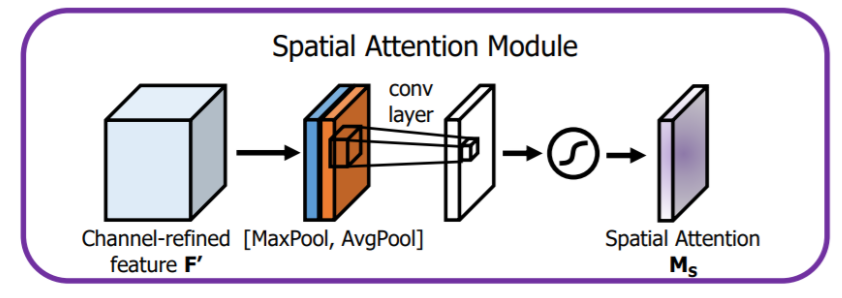
3.空间注意力模块
空间注意力聚焦在“哪里”是最具信息量的部分。计算空间注意力的方法是沿着通道轴应用平均池化和最大池操作,然后将它们连接起来生成一个有效的特征描述符。
import paddle
import paddle.nn as nn

# 空间注意力机制
class SAM_Module(nn.Layer):
    def __init__(self):
        super(SAM_Module, self).__init__()
        self.conv_after_concat = nn.Conv2D(in_channels=2, out_channels=1, kernel_size=7, stride=1, padding=3)
        self.sigmoid_spatial = nn.Sigmoid()

    def forward(self, x):
        # Spatial Attention Module
        module_input = x
        avg = paddle.mean(x, axis=1, keepdim=True)
        mx = paddle.argmax(x, axis=1, keepdim=True)
        mx = paddle.cast(mx, 'float32')
        x = paddle.concat([avg, mx], axis=1)
        x = self.conv_after_concat(x)
        x = self.sigmoid_spatial(x)
        x = module_input * x

        return x
4.搭建SAM-GoogLeNet-BN
class SAM_GoogLeNet_BN(nn.Layer):
    def __init__(self, num_keypoints=68):
        super(SAM_GoogLeNet_BN, self).__init__()

        self.relu = nn.ReLU()
        self.bn64 = nn.BatchNorm(num_channels=64)
        self.bn192 = nn.BatchNorm(192)
        self.bn256 = nn.BatchNorm(256)
        self.bn480 = nn.BatchNorm(480)
        self.bn512 = nn.BatchNorm(512)
        self.bn528 = nn.BatchNorm(528)
        self.bn832 = nn.BatchNorm(832)
        self.bn1024 = nn.BatchNorm(1024)

        self.conv1 = nn.Conv2D(in_channels=3, out_channels=64, kernel_size=7, padding=3, stride=2, data_format='NCHW')
        self.SAM_Module1 = SAM_Module()
        self.pool1 = nn.MaxPool2D(kernel_size=3, stride=2, padding=1)
        self.conv2_1 = nn.Conv2D(64, 64, 1,)
        self.conv2_2 = nn.Conv2D(64, 192, 3, padding=1)

        self.SAM_Module2 = SAM_Module()
        self.pool2 = nn.MaxPool2D(kernel_size=3, stride=2, padding=1)
        self.block3_a = Inception((192, 64), (96, 128), (16, 32), 32)
        self.block3_b = Inception((256, 128), (128, 192), (32, 96), 64)

        self.SAM_Module3 = SAM_Module()
        self.pool3 = nn.MaxPool2D(kernel_size=3, stride=2, padding=1)
        self.block4_a = Inception((480, 192), (96, 208), (16, 48), 64)
        self.block4_b = Inception((512, 160), (112, 224), (24, 64), 64)
        self.block4_c = Inception((512, 128), (128, 256), (24, 64), 64)
        self.block4_d = Inception((512, 112), (144, 288), (32, 64), 64)
        self.block4_e = Inception((528, 256), (160, 320), (32, 128), 128)

        self.SAM_Module4 = SAM_Module()
        self.pool4 = nn.MaxPool2D(kernel_size=3, stride=2, padding=1)
        self.block5_a = Inception((832, 256), (160, 320), (32, 128), 128)
        self.block5_b = Inception((832, 384), (192, 384), (48, 128), 128)
        self.pool5 = nn.AvgPool2D(kernel_size=7, stride=1)
        self.drop = nn.Dropout(0.2)
        self.fc1 = nn.Linear(1024, 512)
        self.fc2 = nn.Linear(512, num_keypoints * 2)

    # 网络的前向计算过程
    def forward(self, x):
        x = self.conv1(x)
        x = self.relu(x)

        x = self.SAM_Module1(x)
        x = self.relu(self.conv2_2(self.relu(self.conv2_1(self.bn64(self.pool1(x))))))

        x = self.SAM_Module2(x)
        x = self.block3_b(self.block3_a(self.bn192(self.pool2(x))))

        x = self.SAM_Module3(x)
        x = self.block4_e(self.block4_d(self.block4_c(self.block4_b(self.block4_a(self.bn480(self.pool3(x)))))))

        x = self.SAM_Module4(x)
        x = self.bn1024(self.pool5(self.block5_b(self.block5_a(self.bn832(self.pool4(x))))))

        x = self.drop(x)
        x = fluid.layers.reshape(x, [-1, 1024])
        x = self.fc1(x)
        x = self.relu(x)
        x = self.fc2(x)

        return x
5.网络结构可视化
使用model.summary查看网络结构。
model = paddle.Model(SAM_GoogLeNet_BN(num_keypoints=68))
model.summary((1, 3, 224, 224))
---------------------------------------------------------------------------
 Layer (type)       Input Shape          Output Shape         Param #
===========================================================================
  Conv2D-1239    [[1, 3, 224, 224]]   [1, 64, 112, 112]        9,472
   ReLU-1010         [[1, 512]]            [1, 512]              0
  Conv2D-1240    [[1, 2, 112, 112]]    [1, 1, 112, 112]         99
  Sigmoid-36     [[1, 1, 112, 112]]    [1, 1, 112, 112]          0
 SAM_Module-36  [[1, 64, 112, 112]]   [1, 64, 112, 112]          0
 MaxPool2D-61   [[1, 64, 112, 112]]    [1, 64, 56, 56]           0
 BatchNorm-225   [[1, 64, 56, 56]]     [1, 64, 56, 56]          256
  Conv2D-1241    [[1, 64, 56, 56]]     [1, 64, 56, 56]         4,160
  Conv2D-1242    [[1, 64, 56, 56]]     [1, 192, 56, 56]       110,784
  Conv2D-1243     [[1, 2, 56, 56]]      [1, 1, 56, 56]          99
  Sigmoid-37      [[1, 1, 56, 56]]      [1, 1, 56, 56]           0
 SAM_Module-37   [[1, 192, 56, 56]]    [1, 192, 56, 56]          0
 MaxPool2D-62    [[1, 192, 56, 56]]    [1, 192, 28, 28]          0
 BatchNorm-226   [[1, 192, 28, 28]]    [1, 192, 28, 28]         768
  Conv2D-1244    [[1, 192, 28, 28]]    [1, 64, 28, 28]        12,352
   ReLU-1011     [[1, 32, 28, 28]]     [1, 32, 28, 28]           0
  Conv2D-1245    [[1, 192, 28, 28]]    [1, 96, 28, 28]        18,528
  Conv2D-1246    [[1, 96, 28, 28]]     [1, 128, 28, 28]       110,720
  Conv2D-1247    [[1, 192, 28, 28]]    [1, 16, 28, 28]         3,088
  Conv2D-1248    [[1, 16, 28, 28]]     [1, 32, 28, 28]        12,832
 MaxPool2D-63    [[1, 192, 28, 28]]    [1, 192, 28, 28]          0
  Conv2D-1249    [[1, 192, 28, 28]]    [1, 32, 28, 28]         6,176
 Inception-82    [[1, 192, 28, 28]]    [1, 256, 28, 28]          0
  Conv2D-1250    [[1, 256, 28, 28]]    [1, 128, 28, 28]       32,896
   ReLU-1012     [[1, 64, 28, 28]]     [1, 64, 28, 28]           0
  Conv2D-1251    [[1, 256, 28, 28]]    [1, 128, 28, 28]       32,896
  Conv2D-1252    [[1, 128, 28, 28]]    [1, 192, 28, 28]       221,376
  Conv2D-1253    [[1, 256, 28, 28]]    [1, 32, 28, 28]         8,224
  Conv2D-1254    [[1, 32, 28, 28]]     [1, 96, 28, 28]        76,896
 MaxPool2D-64    [[1, 256, 28, 28]]    [1, 256, 28, 28]          0
  Conv2D-1255    [[1, 256, 28, 28]]    [1, 64, 28, 28]        16,448
 Inception-83    [[1, 256, 28, 28]]    [1, 480, 28, 28]          0
  Conv2D-1256     [[1, 2, 28, 28]]      [1, 1, 28, 28]          99
  Sigmoid-38      [[1, 1, 28, 28]]      [1, 1, 28, 28]           0
 SAM_Module-38   [[1, 480, 28, 28]]    [1, 480, 28, 28]          0
 MaxPool2D-65    [[1, 480, 28, 28]]    [1, 480, 14, 14]          0
 BatchNorm-228   [[1, 480, 14, 14]]    [1, 480, 14, 14]        1,920
  Conv2D-1257    [[1, 480, 14, 14]]    [1, 192, 14, 14]       92,352
   ReLU-1013     [[1, 64, 14, 14]]     [1, 64, 14, 14]           0
  Conv2D-1258    [[1, 480, 14, 14]]    [1, 96, 14, 14]        46,176
  Conv2D-1259    [[1, 96, 14, 14]]     [1, 208, 14, 14]       179,920
  Conv2D-1260    [[1, 480, 14, 14]]    [1, 16, 14, 14]         7,696
  Conv2D-1261    [[1, 16, 14, 14]]     [1, 48, 14, 14]        19,248
 MaxPool2D-66    [[1, 480, 14, 14]]    [1, 480, 14, 14]          0
  Conv2D-1262    [[1, 480, 14, 14]]    [1, 64, 14, 14]        30,784
 Inception-84    [[1, 480, 14, 14]]    [1, 512, 14, 14]          0
  Conv2D-1263    [[1, 512, 14, 14]]    [1, 160, 14, 14]       82,080
   ReLU-1014     [[1, 64, 14, 14]]     [1, 64, 14, 14]           0
  Conv2D-1264    [[1, 512, 14, 14]]    [1, 112, 14, 14]       57,456
  Conv2D-1265    [[1, 112, 14, 14]]    [1, 224, 14, 14]       226,016
  Conv2D-1266    [[1, 512, 14, 14]]    [1, 24, 14, 14]        12,312
  Conv2D-1267    [[1, 24, 14, 14]]     [1, 64, 14, 14]        38,464
 MaxPool2D-67    [[1, 512, 14, 14]]    [1, 512, 14, 14]          0
  Conv2D-1268    [[1, 512, 14, 14]]    [1, 64, 14, 14]        32,832
 Inception-85    [[1, 512, 14, 14]]    [1, 512, 14, 14]          0
  Conv2D-1269    [[1, 512, 14, 14]]    [1, 128, 14, 14]       65,664
   ReLU-1015     [[1, 64, 14, 14]]     [1, 64, 14, 14]           0
  Conv2D-1270    [[1, 512, 14, 14]]    [1, 128, 14, 14]       65,664
  Conv2D-1271    [[1, 128, 14, 14]]    [1, 256, 14, 14]       295,168
  Conv2D-1272    [[1, 512, 14, 14]]    [1, 24, 14, 14]        12,312
  Conv2D-1273    [[1, 24, 14, 14]]     [1, 64, 14, 14]        38,464
 MaxPool2D-68    [[1, 512, 14, 14]]    [1, 512, 14, 14]          0
  Conv2D-1274    [[1, 512, 14, 14]]    [1, 64, 14, 14]        32,832
 Inception-86    [[1, 512, 14, 14]]    [1, 512, 14, 14]          0
  Conv2D-1275    [[1, 512, 14, 14]]    [1, 112, 14, 14]       57,456
   ReLU-1016     [[1, 64, 14, 14]]     [1, 64, 14, 14]           0
  Conv2D-1276    [[1, 512, 14, 14]]    [1, 144, 14, 14]       73,872
  Conv2D-1277    [[1, 144, 14, 14]]    [1, 288, 14, 14]       373,536
  Conv2D-1278    [[1, 512, 14, 14]]    [1, 32, 14, 14]        16,416
  Conv2D-1279    [[1, 32, 14, 14]]     [1, 64, 14, 14]        51,264
 MaxPool2D-69    [[1, 512, 14, 14]]    [1, 512, 14, 14]          0
  Conv2D-1280    [[1, 512, 14, 14]]    [1, 64, 14, 14]        32,832
 Inception-87    [[1, 512, 14, 14]]    [1, 528, 14, 14]          0
  Conv2D-1281    [[1, 528, 14, 14]]    [1, 256, 14, 14]       135,424
   ReLU-1017     [[1, 128, 14, 14]]    [1, 128, 14, 14]          0
  Conv2D-1282    [[1, 528, 14, 14]]    [1, 160, 14, 14]       84,640
  Conv2D-1283    [[1, 160, 14, 14]]    [1, 320, 14, 14]       461,120
  Conv2D-1284    [[1, 528, 14, 14]]    [1, 32, 14, 14]        16,928
  Conv2D-1285    [[1, 32, 14, 14]]     [1, 128, 14, 14]       102,528
 MaxPool2D-70    [[1, 528, 14, 14]]    [1, 528, 14, 14]          0
  Conv2D-1286    [[1, 528, 14, 14]]    [1, 128, 14, 14]       67,712
 Inception-88    [[1, 528, 14, 14]]    [1, 832, 14, 14]          0
  Conv2D-1287     [[1, 2, 14, 14]]      [1, 1, 14, 14]          99
  Sigmoid-39      [[1, 1, 14, 14]]      [1, 1, 14, 14]           0
 SAM_Module-39   [[1, 832, 14, 14]]    [1, 832, 14, 14]          0
 MaxPool2D-71    [[1, 832, 14, 14]]     [1, 832, 7, 7]           0
 BatchNorm-231    [[1, 832, 7, 7]]      [1, 832, 7, 7]         3,328
  Conv2D-1288     [[1, 832, 7, 7]]      [1, 256, 7, 7]        213,248
   ReLU-1018      [[1, 128, 7, 7]]      [1, 128, 7, 7]           0
  Conv2D-1289     [[1, 832, 7, 7]]      [1, 160, 7, 7]        133,280
  Conv2D-1290     [[1, 160, 7, 7]]      [1, 320, 7, 7]        461,120
  Conv2D-1291     [[1, 832, 7, 7]]      [1, 32, 7, 7]         26,656
  Conv2D-1292     [[1, 32, 7, 7]]       [1, 128, 7, 7]        102,528
 MaxPool2D-72     [[1, 832, 7, 7]]      [1, 832, 7, 7]           0
  Conv2D-1293     [[1, 832, 7, 7]]      [1, 128, 7, 7]        106,624
 Inception-89     [[1, 832, 7, 7]]      [1, 832, 7, 7]           0
  Conv2D-1294     [[1, 832, 7, 7]]      [1, 384, 7, 7]        319,872
   ReLU-1019      [[1, 128, 7, 7]]      [1, 128, 7, 7]           0
  Conv2D-1295     [[1, 832, 7, 7]]      [1, 192, 7, 7]        159,936
  Conv2D-1296     [[1, 192, 7, 7]]      [1, 384, 7, 7]        663,936
  Conv2D-1297     [[1, 832, 7, 7]]      [1, 48, 7, 7]         39,984
  Conv2D-1298     [[1, 48, 7, 7]]       [1, 128, 7, 7]        153,728
 MaxPool2D-73     [[1, 832, 7, 7]]      [1, 832, 7, 7]           0
  Conv2D-1299     [[1, 832, 7, 7]]      [1, 128, 7, 7]        106,624
 Inception-90     [[1, 832, 7, 7]]     [1, 1024, 7, 7]           0
  AvgPool2D-7    [[1, 1024, 7, 7]]     [1, 1024, 1, 1]           0
 BatchNorm-232   [[1, 1024, 1, 1]]     [1, 1024, 1, 1]         4,096
  Dropout-22     [[1, 1024, 1, 1]]     [1, 1024, 1, 1]           0
   Linear-22        [[1, 1024]]            [1, 512]           524,800
   Linear-23         [[1, 512]]            [1, 136]           69,768
===========================================================================
Total params: 6,578,884
Trainable params: 6,568,516
Non-trainable params: 10,368
---------------------------------------------------------------------------
Input size (MB): 0.57
Forward/backward pass size (MB): 64.93
Params size (MB): 25.10
Estimated Total Size (MB): 90.60
---------------------------------------------------------------------------

{'total_params': 6578884, 'trainable_params': 6568516}
四、模型训练
1.模型配置
训练模型前,需要设置训练模型所需的优化器,损失函数和评估指标。
- 优化器:Momentum优化器
- 损失函数:SmoothL1Loss
- 评估指标:NME
2.自定义评估指标
特定任务的 Metric 计算方式在框架既有的 Metric接口中不存在,或算法不符合自己的需求,那么需要我们自己来进行Metric的自定义。这里介绍如何进行Metric的自定义操作,更多信息可以参考官网文档自定义Metric;首先来看下面的代码。
from paddle.metric import Metric

class NME(Metric):
    """
    1. 继承paddle.metric.Metric
    """
    def __init__(self, name='nme', *args, **kwargs):
        """
        2. 构造函数实现,自定义参数即可
        """
        super(NME, self).__init__(*args, **kwargs)
        self._name = name
        self.rmse = 0
        self.sample_num = 0

    def name(self):
        """
        3. 实现name方法,返回定义的评估指标名字
        """
        return self._name

    def update(self, preds, labels):
        """
        4. 实现update方法,用于单个batch训练时进行评估指标计算。
        - 当`compute`类函数未实现时,会将模型的计算输出和标签数据的展平作为`update`的参数传入。
        """
        N = preds.shape[0]

        preds = preds.reshape((N, -1, 2))
        labels = labels.reshape((N, -1, 2))

        self.rmse = 0

        for i in range(N):
            pts_pred, pts_gt = preds[i, ], labels[i, ]
            interocular = np.linalg.norm(pts_gt[36, ] - pts_gt[45, ])

            self.rmse += np.sum(np.linalg.norm(pts_pred - pts_gt, axis=1)) / (interocular * preds.shape[1])
            self.sample_num += 1

        return self.rmse / N

    def accumulate(self):
        """
        5. 实现accumulate方法,返回历史batch训练积累后计算得到的评价指标值。
        每次`update`调用时进行数据积累,`accumulate`计算时对积累的所有数据进行计算并返回。
        结算结果会在`fit`接口的训练日志中呈现。
        """
        return self.rmse / self.sample_num

    def reset(self):
        """
        6. 实现reset方法,每个Epoch结束后进行评估指标的重置,这样下个Epoch可以重新进行计算。
        """
        self.rmse = 0
        self.sample_num = 0
# 调用飞桨框架的VisualDL模块,保存信息到目录中。
callback = paddle.callbacks.VisualDL(log_dir='visualdl_log_dir')

# 定义Momentum优化器
lr = paddle.optimizer.lr.CosineAnnealingDecay(learning_rate=0.01, T_max=len(train_dataset) // 64 * 50)
optimizer = paddle.optimizer.Momentum(learning_rate=lr,
                                     parameters=model.parameters(),
                                     weight_decay=paddle.regularizer.L2Decay(0.002))

# 定义SmoothL1Loss
loss = nn.SmoothL1Loss()

# 使用自定义metrics
metric = NME()

# 模型训练配置
model.prepare(optimizer=optimizer, loss=loss, metrics=metric)
损失函数的选择:L1Loss、L2Loss、SmoothL1Loss的对比
- L1Loss: 在训练后期,预测值与ground-truth差异较小时, 损失对预测值的导数的绝对值仍然为1,此时如果学习率不变,损失函数将在稳定值附近波动,难以继续收敛达到更高精度。
- L2Loss: 在训练初期,预测值与ground-truth差异较大时,损失函数对预测值的梯度十分大,导致训练不稳定。
- SmoothL1Loss: 在x较小时,对x梯度也会变小,而在x很大时,对x的梯度的绝对值达到上限 1,也不会太大以至于破坏网络参数。
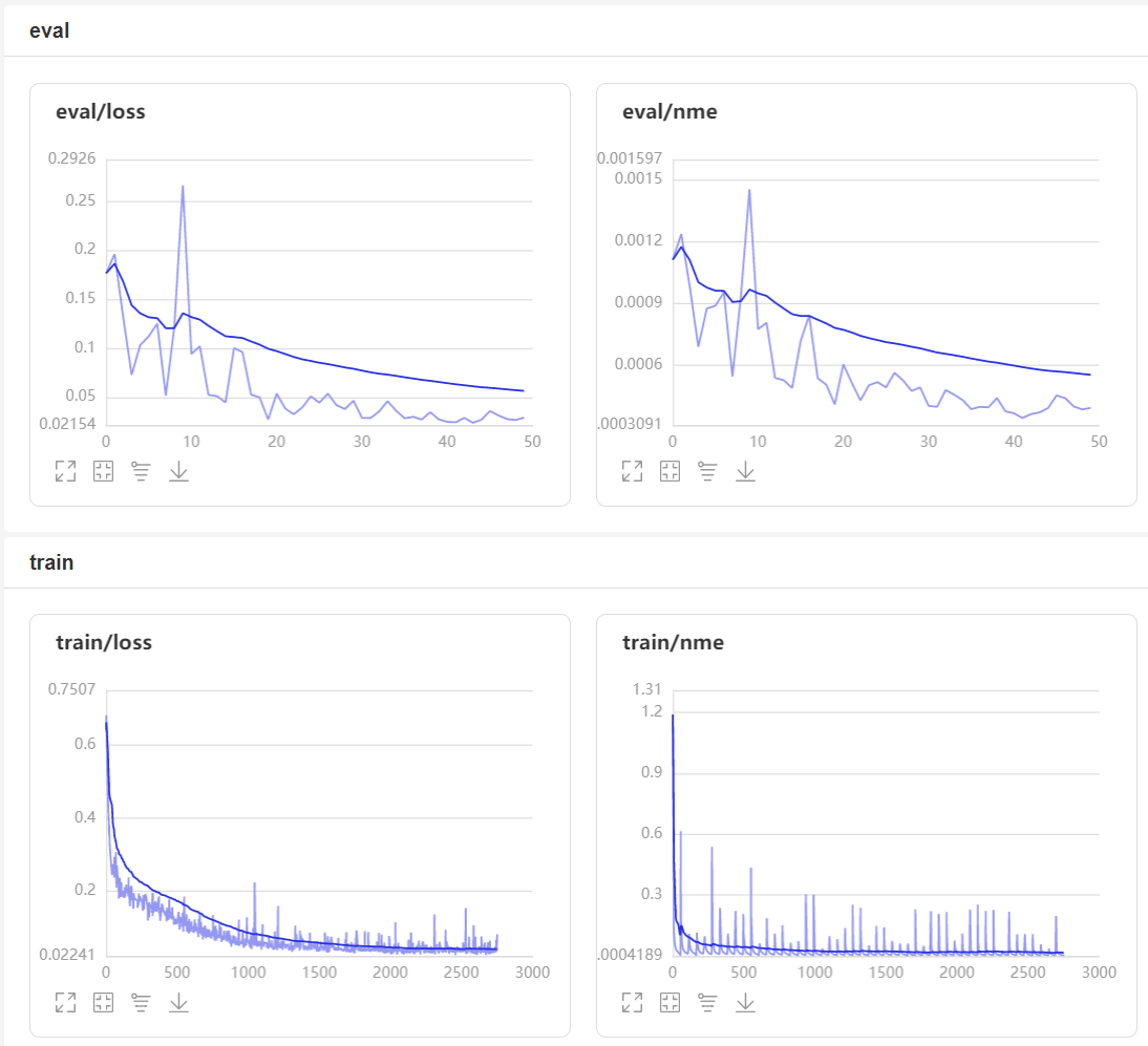
3.模型训练
model.fit(train_dataset,
        test_dataset,
        epochs=50,
        shuffle=True,
        batch_size=64,
        callbacks=callback,
        verbose=1)
The loss value printed in the log is the current step, and the metric is the average value of previous step.
Epoch 1/50
step 55/55 [==============================] - loss: 0.3578 - nme: 0.0013 - 499ms/step
Eval begin...
The loss value printed in the log is the current batch, and the metric is the average value of previous step.
step 13/13 [==============================] - loss: 0.1764 - nme: 0.0011 - 466ms/step
Eval samples: 770
Epoch 2/50
step 55/55 [==============================] - loss: 0.2794 - nme: 0.0013 - 517ms/step
Eval begin...
The loss value printed in the log is the current batch, and the metric is the average value of previous step.
step 13/13 [==============================] - loss: 0.1960 - nme: 0.0012 - 425ms/step
Eval samples: 770
Epoch 3/50
step 55/55 [==============================] - loss: 0.1871 - nme: 0.0010 - 483ms/step
Eval begin...
The loss value printed in the log is the current batch, and the metric is the average value of previous step.
step 13/13 [==============================] - loss: 0.1321 - nme: 9.8054e-04 - 419ms/step
Eval samples: 770
Epoch 4/50
step 55/55 [==============================] - loss: 0.2032 - nme: 9.5976e-04 - 501ms/step
Eval begin...
The loss value printed in the log is the current batch, and the metric is the average value of previous step.
step 13/13 [==============================] - loss: 0.0729 - nme: 6.8905e-04 - 404ms/step
Eval samples: 770
4.模型保存
checkpoints_path = 'work/models'
model.save(checkpoints_path, training=False)
五、模型预测
# 定义功能函数

def show_all_keypoints(image, predicted_key_pts):
    """
    展示图像,预测关键点
    Args:
        image:裁剪后的图像 [224, 224, 3]
        predicted_key_pts: 预测关键点的坐标
    """
    # 展示图像
    plt.imshow(image.astype('uint8'))

    # 展示关键点
    for i in range(0, len(predicted_key_pts), 2):
        plt.scatter(predicted_key_pts[i], predicted_key_pts[i+1], s=20, marker='.', c='m')

def visualize_output(test_images, test_outputs, batch_size=1, h=20, w=10):
    """
    展示图像,预测关键点
    Args:
        test_images:裁剪后的图像 [224, 224, 3]
        test_outputs: 模型的输出
        batch_size: 批大小
        h: 展示的图像高
        w: 展示的图像宽
    """

    if len(test_images.shape) == 3:
        test_images = np.array([test_images])

    for i in range(batch_size):

        plt.figure(figsize=(h, w))
        ax = plt.subplot(1, batch_size, i+1)

        # 随机裁剪后的图像
        image = test_images[i]

        # 模型的输出,未还原的预测关键点坐标值
        predicted_key_pts = test_outputs[i]

        # 还原后的真实的关键点坐标值
        predicted_key_pts = predicted_key_pts * data_std + data_mean

        # 展示图像和关键点
        show_all_keypoints(np.squeeze(image), predicted_key_pts)

        plt.axis('off')

    plt.show()
# 读取图像
img = mpimg.imread('zbp.jpg')

# 关键点占位符
kpt = np.ones((136, 1))

transform = Compose([Resize(256), RandomCrop(224)])

# 对图像先重新定义大小,并裁剪到 224*224的大小
rgb_img, kpt = transform([img, kpt])

norm = GrayNormalize()
to_chw = ToCHW()

# 对图像进行归一化和格式变换
img, kpt = norm([rgb_img, kpt])
img, kpt = to_chw([img, kpt])

img = np.array([img], dtype='float32')

# 加载保存好的模型进行预测
# model = paddle.Model(SAM_GoogLeNet_BN(num_keypoints=68))
# model.load(checkpoints_path)
# model.prepare()

# 预测结果
out = model.predict_batch([img])
out = out[0].reshape((out[0].shape[0], 136, -1))

# 可视化
visualize_output(rgb_img, out, batch_size=1)

六、趣味应用
当我们得到关键点的信息后,就可以进行一些趣味的应用。
1.使用自己训练的模型
def read_image(img_path):
    # 读取图像
    img = mpimg.imread(img_path)

    # 关键点占位符
    kpt = np.ones((136, 1))

    transform = Compose([Resize(256), RandomCrop(224)])

    # 对图像先重新定义大小,并裁剪到 224*224的大小
    rgb_img, kpt = transform([img, kpt])

    norm = GrayNormalize()
    to_chw = ToCHW()

    # 对图像进行归一化和格式变换
    img, kpt = norm([rgb_img, kpt])
    img, kpt = to_chw([img, kpt])

    img = np.array([img], dtype='float32')

    return img
# 定义功能函数
def show_fu(image, predicted_key_pts):
    """
    展示加了贴纸的图像
    Args:
        image:裁剪后的图像 [224, 224, 3]
        predicted_key_pts: 预测关键点的坐标
    """
    # 计算坐标,15 和 34点的中间值
    x = (int(predicted_key_pts[28]) + int(predicted_key_pts[66]))//2
    y = (int(predicted_key_pts[29]) + int(predicted_key_pts[67]))//2

    # 打开 春节小图
    star_image = mpimg.imread('light.jpg')

    # 处理通道
    if(star_image.shape[2] == 4):
        star_image = star_image[:,:,1:4]

    # 将春节小图放到原图上
    image[y:y+len(star_image[0]), x:x+len(star_image[1]),:] = star_image

    # 展示处理后的图片
    plt.imshow(image.astype('uint8'))

    # 展示关键点信息
    for i in range(len(predicted_key_pts)//2,):
        plt.scatter(predicted_key_pts[i*2], predicted_key_pts[i*2+1], s=20, marker='.', c='m') # 展示关键点信息

def custom_output(test_images, test_outputs, batch_size=1, h=20, w=10):
    """
    展示图像,预测关键点
    Args:
        test_images:裁剪后的图像 [224, 224, 3]
        test_outputs: 模型的输出
        batch_size: 批大小
        h: 展示的图像高
        w: 展示的图像宽
    """

    if len(test_images.shape) == 3:
        test_images = np.array([test_images])

    for i in range(batch_size):

        plt.figure(figsize=(h, w))
        ax = plt.subplot(1, batch_size, i+1)

        # 随机裁剪后的图像
        image = test_images[i]

        # 模型的输出,未还原的预测关键点坐标值
        predicted_key_pts = test_outputs[i]

        # 还原后的真实的关键点坐标值
        predicted_key_pts = predicted_key_pts * data_std + data_mean

        # 展示图像和关键点
        show_fu(np.squeeze(image), predicted_key_pts)

        plt.axis('off')

    plt.show()

# 读取图像
img = read_image('zbp.jpg')

# 加载保存好的模型进行预测
# model = paddle.Model(SAM_GoogLeNet_BN(num_keypoints=68))
# model.load(checkpoints_path)
# model.prepare()

# 预测结果
out = model.predict_batch([img])
out = out[0].reshape((out[0].shape[0], 136, -1))

# 可视化
custom_output(rgb_img, out, batch_size=1)

2.使用PaddleHub内置模型
import cv2
import paddlehub as hub
import matplotlib.pyplot as plt
import matplotlib.image as mpimg
import numpy as np
import math
%matplotlib inline

hub.logger.setLevel('ERROR')

src_img = cv2.imread('xiaogege.jpg')

module = hub.Module(name="face_landmark_localization")
result = module.keypoint_detection(images=[src_img])

tmp_img = src_img.copy()
for index, point in enumerate(result[0]['data'][0]):
	# print(point)
	# cv2.putText(img, str(index), (int(point[0]), int(point[1])), cv2.FONT_HERSHEY_COMPLEX, 3, (0,0,255), -1)
	cv2.circle(tmp_img, (int(point[0]), int(point[1])), 2, (0, 0, 255), -1)

res_img_path = 'face_landmark.jpg'
cv2.imwrite(res_img_path, tmp_img)

img = mpimg.imread(res_img_path)
# 展示预测68个关键点结果
plt.figure(figsize=(10,10))
plt.imshow(img)
plt.axis('off')
plt.show()

import os
import paddlehub as hub
import matplotlib.animation as animation
from IPython.display import HTML
from math import degrees, atan2

def overlay_transparent(background_img, img_to_overlay_t, x, y, overlay_size=None):
    bg_img = background_img.copy()
    # convert 3 channels to 4 channels
    if bg_img.shape[2] == 3:
        bg_img = cv2.cvtColor(bg_img, cv2.COLOR_BGR2BGRA)

    if overlay_size is not None:
        img_to_overlay_t = cv2.resize(img_to_overlay_t.copy(), overlay_size)

    b, g, r, a = cv2.split(img_to_overlay_t)

    mask = cv2.medianBlur(a, 5)

    h, w, _ = img_to_overlay_t.shape
    roi = bg_img[int(y - h / 2):int(y + h / 2), int(x - w / 2):int(x + w / 2)]

    img1_bg = cv2.bitwise_and(roi.copy(), roi.copy(), mask=cv2.bitwise_not(mask))
    img2_fg = cv2.bitwise_and(img_to_overlay_t, img_to_overlay_t, mask=mask)

    bg_img[int(y - h / 2):int(y + h / 2), int(x - w / 2):int(x + w / 2)] = cv2.add(img1_bg, img2_fg)

    # convert 4 channels to 3 channels
    bg_img = cv2.cvtColor(bg_img, cv2.COLOR_BGRA2BGR)

    return bg_img

def angle_between(p1, p2):
    x_diff = p2[0] - p1[0]
    y_diff = p2[1] - p1[1]
    return degrees(atan2(y_diff, x_diff))

def get_eye_center_point(landmarks, idx1, idx2):
    center_x = (landmarks[idx1][0] + landmarks[idx2][0]) // 2
    center_y = (landmarks[idx1][1] + landmarks[idx2][1]) // 2
    return (center_x, center_y)

def wear_glasses(image, glasses, eye_left_center, eye_right_center):
    eye_left_center = np.array(eye_left_center)
    eye_right_center = np.array(eye_right_center)
    glasses_center = np.mean([eye_left_center, eye_right_center], axis=0)  # put glasses's center to this center
    glasses_size = np.linalg.norm(eye_left_center - eye_right_center) * 2  # the width of glasses mask
    angle = -angle_between(eye_left_center, eye_right_center)

    glasses_h, glasses_w = glasses.shape[:2]
    glasses_c = (glasses_w / 2, glasses_h / 2)
    M = cv2.getRotationMatrix2D(glasses_c, angle, 1)
    cos = np.abs(M[0, 0])
    sin = np.abs(M[0, 1])

    # compute the new bounding dimensions of the image
    nW = int((glasses_h * sin) + (glasses_w * cos))
    nH = int((glasses_h * cos) + (glasses_w * sin))

    # adjust the rotation matrix to take into account translation
    M[0, 2] += (nW / 2) - glasses_c[0]
    M[1, 2] += (nH / 2) - glasses_c[1]

    rotated_glasses = cv2.warpAffine(glasses, M, (nW, nH))

    try:
        image = overlay_transparent(image, rotated_glasses, glasses_center[0], glasses_center[1],
                                    overlay_size=(
                                        int(glasses_size),
                                        int(rotated_glasses.shape[0] * glasses_size / rotated_glasses.shape[1]))
                                    )
    except:
        print('failed overlay image')
    return image

glasses_lists = []
fig = plt.figure(figsize=(10, 8))
module = hub.Module(name="face_landmark_localization")

for i, path in enumerate(os.listdir('glasses')):
    image_file = 'xiaogege.jpg'
    glasses_file = 'glasses/' + path

    image = cv2.imread(image_file)
    glasses = cv2.imread(glasses_file, cv2.IMREAD_UNCHANGED)
    result = module.keypoint_detection(images=[image])
    landmarks = result[0]['data'][0]
    eye_left_point = get_eye_center_point(landmarks, 36, 39)
    eye_right_point = get_eye_center_point(landmarks, 42, 45)
    image = wear_glasses(image, glasses, eye_left_point, eye_right_point)
    cv2.imwrite(f'result/{i}.png', image)
    image = cv2.cvtColor(image, cv2.COLOR_RGB2BGR)
    im = plt.imshow(image, animated=True)
    plt.axis('off')
    glasses_lists.append([im])

ani = animation.ArtistAnimation(fig, glasses_lists, interval=1000, blit=True, repeat_delay=1000)
.png', image)
    image = cv2.cvtColor(image, cv2.COLOR_RGB2BGR)
    im = plt.imshow(image, animated=True)
    plt.axis('off')
    glasses_lists.append([im])

ani = animation.ArtistAnimation(fig, glasses_lists, interval=1000, blit=True, repeat_delay=1000)
HTML(ani.to_html5_video())

个人简介
北京联合大学 机器人学院 自动化专业 2018级 本科生 郑博培
百度飞桨开发者技术专家 PPDE
百度飞桨官方帮帮团、答疑团成员
深圳柴火创客空间 认证会员
百度大脑 智能对话训练师
我在AI Studio上获得至尊等级,点亮8个徽章,来互关呀!!!
https://aistudio.baidu.com/aistudio/personalcenter/thirdview/147378


 2889
2889


 被折叠的 条评论
为什么被折叠?
被折叠的 条评论
为什么被折叠?
 到【灌水乐园】发言


