【图像处理】 仿射变换（Affine Transformation）和透视变换（Perspective Transformation）

齐次坐标系

欧式空间中，使用用笛卡尔坐标系，对应的，在透视空间中，使用齐次坐标系。

齐次坐标用$n+1$维，对应表示笛卡尔坐标的$n$维，比如：

笛卡尔坐标中的$(x,y)$对应齐次坐标中的$(x_1,y_1,w)$，有$x=\frac{x_1}{w}$，$y=\frac{y_1}{w}$

笛卡尔坐标中的$(2,3)$对应齐次坐标中的$(2,3,1)$等

特别的，笛卡尔坐标中的$(+\infty ,+\infty )$对应齐次坐标中的$(2,3,0)$等

仿射变换的原理

仿射变换，是一次空间线性变换，或多次不同空间线性变换的组合。经过仿射变换后，直线还是直线，圆弧还是圆弧，互为平行线还是互为平行线，但是，不能保证线段的长度和线段之间的夹角角度不变。

仿射变换的原始空间线性变换包括：
（下面四种仿射变换的原始空间线性变换的示意图来自https://www.cnblogs.com/happystudyeveryday/p/10547316.html，感谢原作者的工作）

1. 平移变换（Translation Transformation）
   
   用笛卡尔坐标系表示：
   $\hat{x}=x+t_x$
   $\hat{y}=y+t_y$
   用齐次坐标系表示：
   $\left[\begin{array}{c}\hat{x}\\ \hat{y}\\ 1\end{array}\right]=\left[\begin{array}{ccc}1& 0& t_x\\ 0& 1& t_y\\ 0& 0& 1\end{array}\right]\ast \left[\begin{array}{c}x\\ y\\ 1\end{array}\right]$

2. 旋转变换（Rotation Transformation）
   
   图形围绕原点顺时针旋转$\theta$弧度
   用笛卡尔坐标系表示：
   $\hat{x}=xcos(\theta )-ysin(\theta )$
   $\hat{y}=xsin(\theta )+ycos(\theta )$
   用齐次坐标系表示：
   $\left[\begin{array}{c}\hat{x}\\ \hat{y}\\ 1\end{array}\right]=\left[\begin{array}{ccc}cos(\theta )& -sin(\theta )& 0\\ sin(\theta )& cos(\theta )& 0\\ 0& 0& 1\end{array}\right]\ast \left[\begin{array}{c}x\\ y\\ 1\end{array}\right]$

3. 剪切变换（Shear Transformation ）
   
   用笛卡尔坐标系表示：
   $\hat{x}=x+y\ast t_x$
   $\hat{y}=y+x\ast t_y$
   用齐次坐标系表示：
   $\left[\begin{array}{c}\hat{x}\\ \hat{y}\\ 1\end{array}\right]=\left[\begin{array}{ccc}1& t_x& 0\\ t_y& 1& 0\\ 0& 0& 1\end{array}\right]\ast \left[\begin{array}{c}x\\ y\\ 1\end{array}\right]$

4. 放缩变换（Scale Transformation）
   
   用笛卡尔坐标系表示：
   $\hat{x}=x\ast t_x$
   $\hat{y}=y\ast t_y$
   用齐次坐标系表示：
   $\left[\begin{array}{c}\hat{x}\\ \hat{y}\\ 1\end{array}\right]=\left[\begin{array}{ccc}{t}_x& 0& 0\\ 0& t_y& 0\\ 0& 0& 1\end{array}\right]\ast \left[\begin{array}{c}x\\ y\\ 1\end{array}\right]$

到这里就体现出齐次坐标系的作用了：通过使用齐次坐标系表示，将各种线性空间变换的表示都统一了

所以仿射变换可以表示为：
$\left[\begin{array}{c}\hat{x}\\ \hat{y}\\ 1\end{array}\right]=\left[\begin{array}{ccc}{t}_x& 0& 0\\ 0& t_y& 0\\ 0& 0& 1\end{array}\right]\ast \left[\begin{array}{ccc}1& t_x& 0\\ t_y& 1& 0\\ 0& 0& 1\end{array}\right]\ast \left[\begin{array}{ccc}cos(\theta )& -sin(\theta )& 0\\ sin(\theta )& cos(\theta )& 0\\ 0& 0& 1\end{array}\right]\ast \left[\begin{array}{ccc}1& 0& t_x\\ 0& 1& t_y\\ 0& 0& 1\end{array}\right]\ast \left[\begin{array}{c}x\\ y\\ 1\end{array}\right]$
（注意上式中，不同变换矩阵中的$t_x$、$t_y$不相同）

$\left[\begin{array}{c}\hat{x}\\ \hat{y}\\ 1\end{array}\right]=\left[\begin{array}{ccc}{a}_1& a_2& a_3\\ a_4& a_5& a_6\\ 0& 0& 1\end{array}\right]\ast \left[\begin{array}{c}x\\ y\\ 1\end{array}\right]$

故，仿射变换的变换矩阵有六个自由度，至少需要三对对应点求得。

OpenCV中的仿射变换

1. 根据三个对应点，求得仿射变换矩阵

M = cv2.getAffineTransform(src, dst)

• M：仿射变换矩阵
• src：原始图像中的三个点的坐标
• dst：变换后得到图像中对应的三个点的坐标

2. 根据仿射变换矩阵，将图像进行仿射变换

dst = cv2.warpAffine(src, M, dsize)

• dst：仿射变换后得到的图像
• src：原始图像
• M：仿射变换矩阵
• dsize：仿射变换得到图像的size（注意和resize操作的差别）

仿射变换的部分应用

# -*- coding:utf-8 -*-

import cv2
import numpy as np

img = cv2.imread("test_image.jpg")

cv2.circle(img, (185, 330), 3, (0, 0, 213), -1)
cv2.circle(img, (285, 135), 3, (0, 0, 213), -1)

cv2.imshow("input", img)
cv2.waitKey(0)

kp2 = np.array([285.0, 135.0])
kp0 = np.array([185.0, 330.0])

dir_v = kp2 - kp0

# 两个关键点之间的距离
dist = np.linalg.norm(dir_v)

dir_v /= np.linalg.norm(dir_v)
R90 = np.r_[[[0, 1], [-1, 0]]]

dir_v_r = dir_v @ R90.T

a = np.float32([kp2, kp2 + dir_v*dist, kp2 + dir_v_r*dist])

b = np.float32([
    [int(dist), int(dist)],
    [int(dist), 0],
    [0, int(dist)]])

Mtr = cv2.getAffineTransform(a, b)

img_ = cv2.warpAffine(img, Mtr, (500, 500))

cv2.imshow("output", img_)
cv2.waitKey(0)

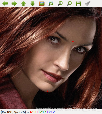输入图像
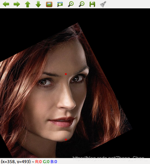仿射变换后得到的图像

透视变换的原理

透视变换，又叫单应性变换。
简而言之就是不同视角的同一物体，在像素坐标系中的变换。

对于齐次坐标系，有：
$\left[\begin{array}{c}\hat{x}\\ \hat{y}\\ 1\end{array}\right]=\left[\begin{array}{ccc}{h}_1& h_2& h_3\\ h_4& h_5& h_6\\ h_7& h_8& h_9\end{array}\right]\ast \left[\begin{array}{c}x\\ y\\ 1\end{array}\right]$

即：
$\hat{x}=h_1\ast x+h_2\ast y+h_3$
$\hat{y}=h_4\ast x+h_5\ast y+h_6$
$1=h_7\ast x+h_8\ast y+h_9$

即：
$\hat{x}=\frac{h_1\ast x+h_2\ast y+h_3}{h_7\ast x+h_8\ast y+h_9}$
$\hat{y}=\frac{h_4\ast x+h_5\ast y+h_6}{h_7\ast x+h_8\ast y+h_9}$

齐次坐标系有性质：
$(\hat{x},\hat{y},1)=(\frac{\hat{x}}{h_9},\frac{y}{h_9},\frac{1}{h_9})$

因此，有：
$\hat{x}=\frac{{h_1}^{/}\ast x+{h_2}^{/}\ast y+{h_3}^{/}}{{h_7}^{/}\ast x+{h_8}^{/}\ast y+1}$
$\hat{y}=\frac{{h_4}^{/}\ast x+{h_5}^{/}\ast y+{h_6}^{/}}{{h_7}^{/}\ast x+{h_8}^{/}\ast y+1}$

故，透视变换的变换矩阵有八个自由度，至少需要四对对应点求得。

OpenCV中的透视变换及应用

# -*- coding:utf-8 -*-

import cv2
import numpy as np
import sys


template_img = cv2.imread("template.jpg")
template_img_gray = cv2.imread("template.jpg", 0)
img = cv2.imread("image.jpg")
img_gray = cv2.imread("image.jpg", 0)

sift = cv2.xfeatures2d.SIFT_create()

# sift算子提取特征
tem_key_points, tem_descriptors = sift.detectAndCompute(template_img_gray, None)
img_key_points, img_descriptors = sift.detectAndCompute(img_gray, None)

# 特征匹配
FLANN_INDEX_KDTREE = 0
index_params = dict(algorithm=FLANN_INDEX_KDTREE, trees=5)
search_params = dict(checks=50)
flann = cv2.FlannBasedMatcher(index_params, search_params)
matches = flann.knnMatch(tem_descriptors, img_descriptors, k=2)

# 去除最好匹配数量不是2的特征匹配
temporary = []
for each in matches:
    if len(each) != 2:
        temporary.append(each)
for each in temporary:
    matches.remove(each)

good_match = []
for i, (m, n) in enumerate(matches):
    if m.distance < 0.9 * n.distance:
        good_match.append(m)

MIN_MATCH_COUNT = 4

if len(good_match) > MIN_MATCH_COUNT:
    src_pts = np.float32([tem_key_points[m.queryIdx].pt for m in good_match]).reshape(-1, 1, 2)
    dst_pts = np.float32([img_key_points[m.trainIdx].pt for m in good_match]).reshape(-1, 1, 2)

    # 计算单应性矩阵
    M, mask = cv2.findHomography(src_pts, dst_pts, cv2.RANSAC, 3.0)
    match_mask = mask.ravel().tolist()

    draw_params = dict(matchColor=(0, 255, 0), singlePointColor=None, matchesMask=match_mask, flags=2)
    match_image = cv2.drawMatches(template_img_gray, tem_key_points, img_gray, img_key_points, good_match, None, **draw_params)
    
    cv2.imshow("Match Image", match_image)
    while True:
        if cv2.waitKey(1000 // 12) & 0xff == ord("q"):  # 按q退出
            break
    cv2.destroyAllWindows()

    if M is not None:
        h, w, _ = template_img.shape
        pts = np.float32([[0, 0], [0, h - 1], [w - 1, h - 1], [w - 1, 0]]).reshape(-1, 1, 2)
        rect = cv2.perspectiveTransform(pts, M)
        rect_ = []
        for each in rect.tolist():
            rect_.append([int(each[0][0]), int(each[0][1])])        
        box_image = cv2.polylines(img, [np.array(rect_)], True, (255, 0, 255), 3, cv2.LINE_AA)

        cv2.imshow("Box Image", box_image)
        while True:
            if cv2.waitKey(1000 // 12) & 0xff == ord("q"):  # 按q退出
                break
        cv2.destroyAllWindows()
    else:
        sys.exit(0)

else:
    sys.exit(0)

模板

测试图片

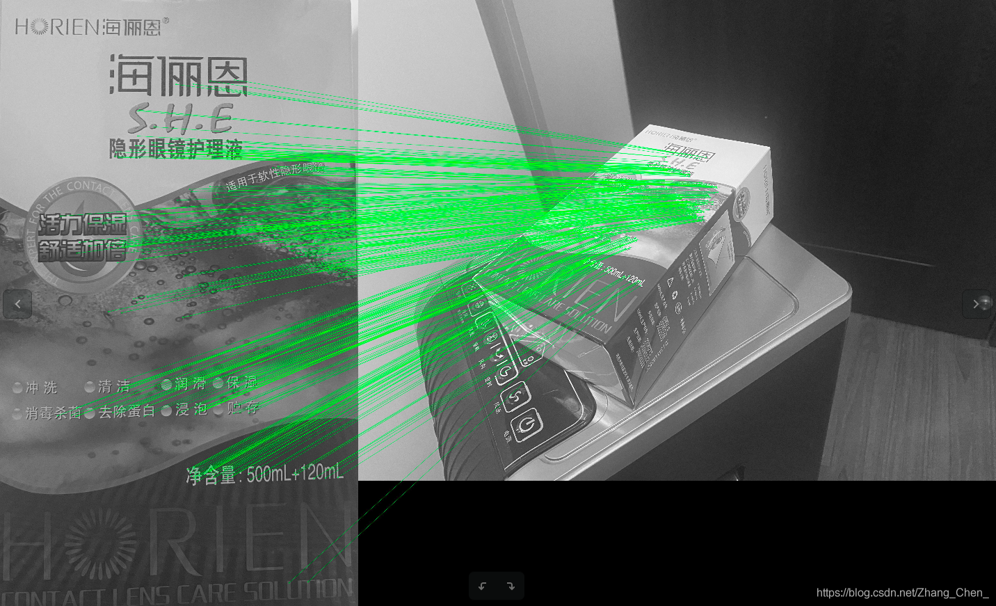
匹配图

通过单应性矩阵得到的检测框

结语

如果您有修改意见或问题，欢迎留言或者通过邮箱和我联系。
手打很辛苦，如果我的文章对您有帮助，转载请注明出处。