


notebooks-master\docs\tutorial_notebooks\DL2\Bayesian_Neural_Networks
贝叶斯神经网络(Bayesian Neural Networks, BNN)和几种不确定性量化方法的教程,包括局部集成(Deep Ensemble)、蒙特卡洛dropout(Monte Carlo Dropout)和一致性预测(Conformal Prediction)。下面是对这段文字的中文解读:
2: 与其他不确定性量化方法的比较
这个教程将探讨贝叶斯神经网络(BNN)相比传统点估计神经网络的优势,并查看其他量化不确定性的方法,包括一致性预测。
导入标准库和设置随机种子以确保可重复性。
模拟数据
让我们模拟一个波动的线条,并在分离的区域中绘制观测数据...
定义非贝叶斯神经网络
首先,创建一个点估计神经网络,换句话说,就是一个标准的全连接多层感知机(MLP)。我们将动态定义隐藏层的数量,以便我们可以为不同深度重用相同的类。
训练一个确定性NN
现在,让我们使用上面生成的训练数据来训练我们的MLP:
评估
让我们研究一下我们的确定性MLP是如何泛化到我们输入变量x的整个域的(模型仅在观测数据上训练,现在我们还将传入此区域外的数据)。
深度集成
深度集成由Lakshminarayanan等人在2017年首次引入。顾名思义,训练多个点估计NN,形成一个集成,最终预测是跨模型的平均值。
蒙特卡罗Dropout
首先,我们创建我们的MC-Dropout网络。正如下面代码所示,创建一个dropout网络非常简单:我们可以重用我们现有的网络架构,唯一的改变是在前向传播时我们会随机关闭(归零)输入张量的一些元素。
一致性预测
一致性预测是一种统计不确定性量化方法,最近在机器学习社区中引起了兴趣。它允许我们在不修改预测模型的情况下,构建我们预测周围的统计严格不确定性带。
练习:在MNIST上检测分布偏移
在这个练习中,我们将比较贝叶斯NN和确定性NN在分布偏移检测任务上的表现。我们将通过监测预测熵随着分布逐渐偏移来实现这一点。
本文介绍了几种不同的不确定性量化方法,并通过模拟数据和MNIST数据集上的实验展示了它们在分布偏移检测方面的性能。贝叶斯方法(包括BNN、Deep Ensemble和MC Dropout)提供了关于模型预测的不确定性的度量,而一致性预测方法则提供了一种不同的、基于统计的方法来量化不确定性。这些方法各有优势,选择哪种方法取决于具体的应用场景和数据特性。
最近的
指导
大规模培训模型
- 概观
- 第1.1部分:在单个GPU上训练更大的模型
- 第1.2部分:分析和缩放单GPU转换器模型
- 第2.1部分:JAX分布式计算简介
- 第2.2部分:(完全分片)数据并行性
- 第3.1部分:管道并行性
- 第3.2部分:循环管道
- 第4.1部分:张量平行性
- 第4.2部分:张量并行的异步线性层
- 第4.3部分:张量并行的变压器
- 第5部分:3D并行语言建模
深度学习1 (PYTORCH)
- 教程PyTorch简介
- 教程3:激活函数
- 教程4:优化和初始化
- 教程5:盗梦空间、ResNet和DenseNet
- 教程6:变形金刚和多头注意力
- 教程7:图形神经网络
- 教程8:基于深层能量的生成模型
- 教程9:深度自动编码器
- 教程10:对抗性攻击
- 教程11:标准化图像建模流程
- 教程12:自回归图像建模
- 教程15:视觉变形金刚
- 教程16:元学习-学会学习
- 教程17:使用SimCLR的自我监督对比学习
深度学习1(JAX+亚麻)
- 教程2(JAX):JAX+亚麻介绍
- 教程3 (JAX):激活函数
- 教程4 (JAX):优化和初始化
- 教程5 (JAX):盗梦空间、ResNet和DenseNet
- 教程6 (JAX):变形金刚和多头注意力
- 教程7 (JAX):图形神经网络
- 教程9 (JAX):深度自动编码器
- 教程11 (JAX):图像建模的规范化流程
- 教程12 (JAX):自回归图像建模
- 教程15 (JAX):视觉变形金刚
- 教程17 (JAX):用SimCLR进行自我监督的对比学习
深度学习2
- GDL正则群卷积
- GDL可控CNN
- DPM1 -深度概率模型I
- 深度离散隐变量模型的DPM2 -变分推断
- 深度连续LVMs的DPM 2 -变分推理
- AGM -标准化流程的高级主题- 1x1卷积
- HDL -超参数调优简介
- HDL -多GPU编程简介
- 教程1:使用Pyro的贝叶斯神经网络
- 教程2:与其他不确定性量化方法的比较
- DNN -教程2第一部分:物理学启发的机器学习
- DNN -教程2第二部分:物理学启发的机器学习
- 动态系统和神经微分方程
- SGA采样离散结构
- 具有Gumbel-Top的SGA采样子集k休闲活动
- SGA:用Gumbel-Sinkhorn网络学习潜在排列
- 用于神经关系推理的SGA图采样
- 时间介入序列的CRL因果可识别性
- »
- 教程2:与其他不确定性量化方法的比较
- 在GitHub上编辑
教程2:与其他不确定性量化方法的比较
填满的笔记本:-最新版本(V04/23):这款笔记本电脑
空笔记本:-最新版本(V04/23):

作者:伊尔泽·阿曼达·奥兹纳、伦纳德·贝雷斯卡、亚历山大·蒂曼斯和埃里克·纳利斯尼克
在本教程中,我们将研究贝叶斯神经网络(BNN)相比点估计神经网络有哪些优势。我们还将研究其他不确定性量化方法,包括保形预测。
导入标准库并设置随机种子以获得重现性。
[1]:
import torch
import torch.nn as nn
import numpy as np
import matplotlib.pyplot as plt
from tqdm.auto import trange, tqdm

torch.manual_seed(42)
np.random.seed(42)
模拟数据
让我们模拟一条蜿蜒的线,在不同的区域画出观察结果…
[2]:
def get_simple_data_train():
    x = np.linspace(-.2, 0.2, 500)
    x = np.hstack([x, np.linspace(.6, 1, 500)])
    eps = 0.02 * np.random.randn(x.shape[0])
    y = x + 0.3 * np.sin(2 * np.pi * (x + eps)) + 0.3 * np.sin(4 * np.pi * (x + eps)) + eps
    x_train = torch.from_numpy(x).float()[:, None]
    y_train = torch.from_numpy(y).float()
    return x_train, y_train
[3]:
def plot_generic(add_to_plot=None):
    fig, ax = plt.subplots(figsize=(10, 5))
    plt.xlim([-.5, 1.5])
    plt.ylim([-1.5, 2.5])
    plt.xlabel("X", fontsize=30)
    plt.ylabel("Y", fontsize=30)

    x_train, y_train = get_simple_data_train()

    x_true = np.linspace(-.5, 1.5, 1000)
    y_true = x_true + 0.3 * np.sin(2 * np.pi * x_true) + 0.3 * np.sin(4 * np.pi * x_true)

    ax.plot(x_train, y_train, 'ko', markersize=4, label="observations")
    ax.plot(x_true, y_true, 'b-', linewidth=3, label="true function")
    if add_to_plot is not None:
        add_to_plot(ax)

    plt.legend(loc=4, fontsize=15, frameon=False)
    plt.show()
[4]:
plot_generic()
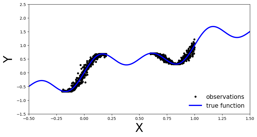
正如你所看到的,我们有蓝色的真函数。观察值在函数的两个区域中是可观察的,并且在它们的测量中存在一些噪声。我们将使用这个简单的数据来展示BNNs和确定性nn之间的差异。
定义非贝叶斯神经网络
首先让我们创建我们的点估计神经网络,换句话说,一个标准的全连接MLP。我们将动态定义隐藏层的数量,这样我们就可以在不同的深度重用同一个类。我们还将添加一个拒绝传统社会的人标志,这将允许我们轻松地为我们的BNN使用相同的架构。
[5]:
class MLP(nn.Module):
    def __init__(self, input_dim=1, output_dim=1, hidden_dim=10, n_hidden_layers=1, use_dropout=False):
        super().__init__()

        self.use_dropout = use_dropout
        if use_dropout:
            self.dropout = nn.Dropout(p=0.5)
        self.activation = nn.Tanh()

        # dynamically define architecture
        self.layer_sizes = [input_dim] + n_hidden_layers * [hidden_dim] + [output_dim]
        layer_list = [nn.Linear(self.layer_sizes[idx - 1], self.layer_sizes[idx]) for idx in
                      range(1, len(self.layer_sizes))]
        self.layers = nn.ModuleList(layer_list)

    def forward(self, input):
        hidden = self.activation(self.layers[0](input))
        for layer in self.layers[1:-1]:
            hidden_temp = self.activation(layer(hidden))

            if self.use_dropout:
                hidden_temp = self.dropout(hidden_temp)

            hidden = hidden_temp + hidden  # residual connection

        output_mean = self.layers[-1](hidden).squeeze()
        return output_mean
训练一个确定性神经网络
培养
现在,让我们用上面生成的训练数据来训练我们的MLP:
[6]:
def train(net, train_data):
    x_train, y_train = train_data
    optimizer = torch.optim.Adam(params=net.parameters(), lr=1e-3)
    criterion = nn.MSELoss()

    progress_bar = trange(3000)
    for _ in progress_bar:
        optimizer.zero_grad()
        loss = criterion(y_train, net(x_train))
        progress_bar.set_postfix(loss=f'{loss / x_train.shape[0]:.3f}')
        loss.backward()
        optimizer.step()
    return net
[7]:
train_data = get_simple_data_train()
x_test = torch.linspace(-.5, 1.5, 3000)[:, None]  # test over the whole range

net = MLP(hidden_dim=30, n_hidden_layers=2)
net = train(net, train_data)
y_preds = net(x_test).clone().detach().numpy()
评价
让我们研究一下确定性MLP是如何在输入变量的整个范围内推广的x(该模型仅根据观察值进行训练,现在我们还将传入该区域以外的数据)
[8]:
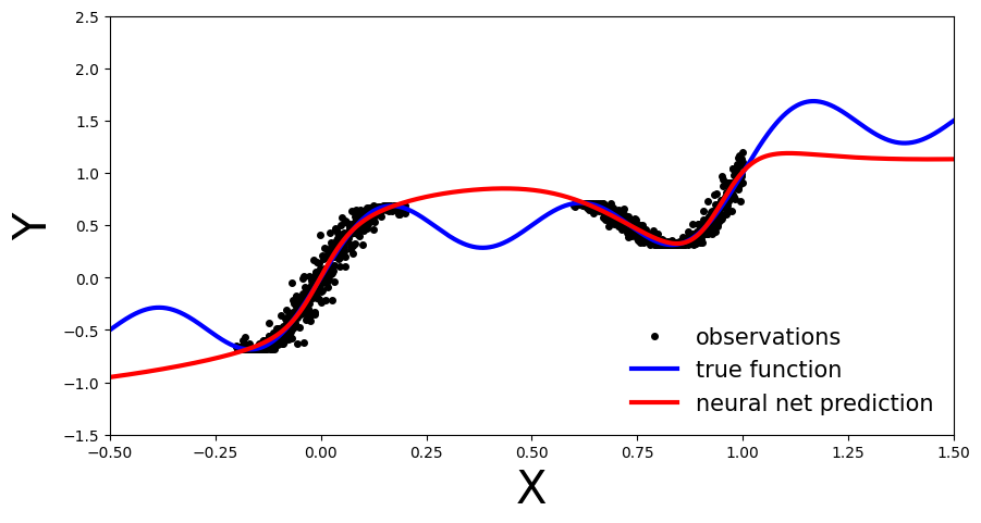
def plot_predictions(x_test, y_preds):
    def add_predictions(ax):
        ax.plot(x_test, y_preds, 'r-', linewidth=3, label='neural net prediction')

    plot_generic(add_predictions)
plot_predictions(x_test, y_preds)
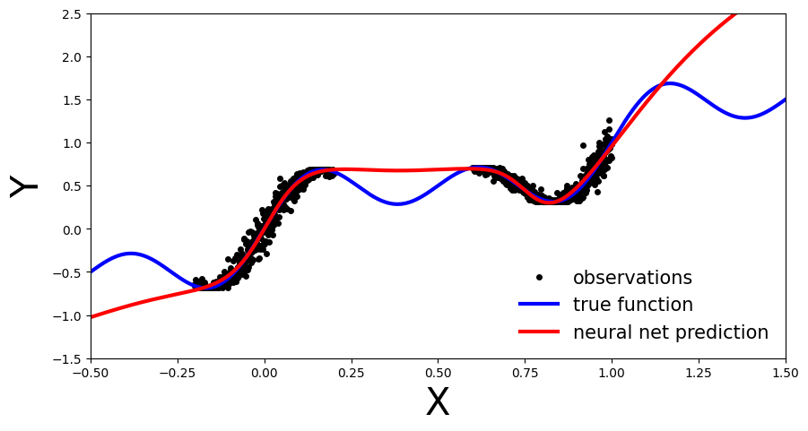
我们可以看到,我们的确定性MLP(红线)已经正确地学习了训练区域中的数据分布,但是,由于模型没有学习基础正弦波函数,所以它在训练区域之外的预测是不准确的。因为我们的MLP是一个点估计NN,所以我们在训练区域之外的预测中没有测量置信度。在接下来的章节中,让我们来看看它与BNN的对比。
深度合奏
深度合奏最早是由Lakshminarayanan等人(2017年)。顾名思义,训练多个点估计NN,合奏,最后的预测是作为所有模型的平均值计算的。从贝叶斯的角度来看,不同的点估计对应于贝叶斯后验模型。这可以解释为用参数化为多个狄拉克δ的分布来近似后验概率:
qϕ(θ|D)=∑θi∈ϕαθiδθi(θ)
在哪里αθi是正常数,使得它们的和等于1。
培养
我们将重用之前介绍的MLP架构,简单地说,现在我们将训练此类模型的集合
[9]:
ensemble_size = 5
ensemble = [MLP(hidden_dim=30, n_hidden_layers=2) for _ in range(ensemble_size)]
for net in ensemble:
    train(net, train_data)
评价
和以前一样,让我们研究我们的深度集成如何在输入变量的整个数据域上执行x.
[10]:
y_preds = [np.array(net(x_test).clone().detach().numpy()) for net in ensemble]
画出每个系综成员的预测函数。
[11]:
def plot_multiple_predictions(x_test, y_preds):
    def add_multiple_predictions(ax):
        for idx in range(len(y_preds)):
            ax.plot(x_test, y_preds[idx], '-', linewidth=3)

    plot_generic(add_multiple_predictions)
[12]:
plot_multiple_predictions(x_test, y_preds)
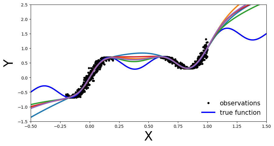
在这个图中,集合方法的好处还不清楚。仍然在训练数据之外的区域,每个被训练的NN是不准确的。你可能会问这有什么好处。
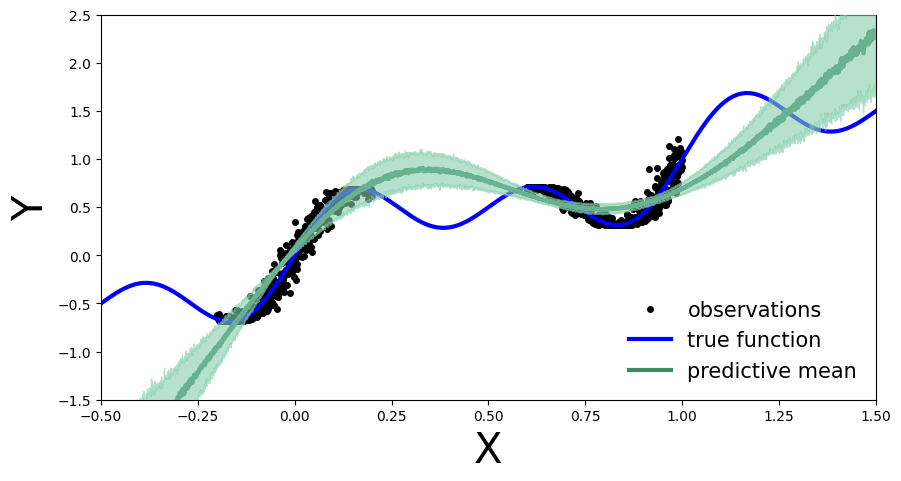
好吧,让我们以稍微不同的方式画出上面的图:让我们想象全体的不确定带。>从贝叶斯的角度来看,我们希望量化模型预测的不确定性。这是通过边缘p(y|x,D),可计算如下:
p(y|x,D)=∫θp(y|x,θ′)p(θ′|D)dθ′Inpractice,forDeepEnsemblesweapproximatetheabovebycomputingthemeanandstandarddeviationacrosstheensemble.Meaning:math:‘p(θ|D)‘representstheparametersofoneofthetrainedmodels,:math:‘θi∼p(θ|D)‘,whichwethenusetocompute:math:‘yi=f(x,θi)‘,representing:math:‘p(y|x,θ′)‘.
[13]:
def plot_uncertainty_bands(x_test, y_preds):
    y_preds = np.array(y_preds)
    y_mean = y_preds.mean(axis=0)
    y_std = y_preds.std(axis=0)

    def add_uncertainty(ax):
        ax.plot(x_test, y_mean, '-', linewidth=3, color="#408765", label="predictive mean")
        ax.fill_between(x_test.ravel(), y_mean - 2 * y_std, y_mean + 2 * y_std, alpha=0.6, color='#86cfac', zorder=5)

    plot_generic(add_uncertainty)
[14]:
plot_uncertainty_bands(x_test, y_preds)

现在我们看到了贝叶斯方法的好处。在训练区域之外,我们不仅有点估计,而且还有模型关于其预测的不确定性。
蒙特卡洛辍学
首先,我们创建我们的MC-Dropout网络。正如您在下面的代码中看到的,创建一个dropout网络非常简单:我们可以重用我们现有的网络架构,唯一的改变是在转发过程中我们随机地切断(零)输入张量的一些元素。
对MC-Dropout的贝叶斯解释是,我们可以将每个Dropout配置视为来自近似后验分布的不同样本θi∼q(θ|D).
培养
[15]:
net_dropout = MLP(hidden_dim=30, n_hidden_layers=2, use_dropout=True)
net_dropout = train(net_dropout, train_data)
评价
类似于深度集成,我们通过MC-Dropout网络多次传递测试数据。我们这样做是为了获得yi在不同的参数设置下,θi网络的一部分,yi=f(x,θi),由漏失掩码控制。
这是与确定性NN中的丢弃实现相比的主要区别,在确定性NN中,丢弃实现用作正则化项。在测试期间的正常压差应用中,压差为不已应用。这意味着所有连接都存在,但是权重调整过的
[16]:
n_dropout_samples = 100

# compute predictions, resampling dropout mask for each forward pass
y_preds = [net_dropout(x_test).clone().detach().numpy() for _ in range(n_dropout_samples)]
y_preds = np.array(y_preds)
[17]:
plot_multiple_predictions(x_test, y_preds)
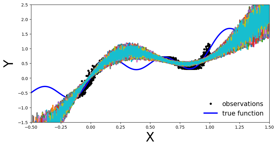
在上面的图中,每条彩色线(除了蓝色)代表不同的参数化,θi我们MC-Dropout网络的。
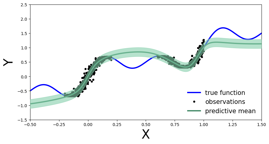
同样,对于深度系综网络,我们也可以计算MC-dropout不确定带.
实践中的方法与之前相同:我们计算每个漏失屏蔽的平均值和标准偏差,这对应于我们之前讨论的边际估计。
[18]:
plot_uncertainty_bands(x_test, y_preds)
与深度集成一样,MC-Dropout允许我们在逐点预测的基础上进行不确定性估计。然而,对于给定的用例,这伴随着模型在训练区域上的整体性能下降的代价。我们观察到这一点,是因为每次通过网络时,我们都会随机选择保留哪些节点,因此有人可能会认为我们阻碍了网络的最佳性能。
保形预测
保形预测是一种统计不确定性量化方法,最近在机器学习社区中引起了兴趣。最初由提出Vovk等人。,它允许我们围绕我们的预测构建统计上严格的不确定性范围,而不需要对我们的预测模型进行任何修改。这是通过比较样本外数据的真实值和预测值来实现的(更准确地说,我们看到的是感应的共形预测),并计算经验分位数q^基于这些比较,定义不确定频带的幅度。我们如何比较真实值和预测值是一个建模决策,有不同的方法可以做到这一点。比较结果也称为(不)符合性分数,因此命名为该方法。
如果我们遵循保形配方,在最小假设的情况下,我们的不确定性带在统计上是严格的,因为它们满足任何测试样品的良好特性(Xn+1,Yn+1):
P(Yn+1∈C^(Xn+1))≥1−α,
即至少有概率1−α,我们计算的不确定带C^(Xn+1)围绕我们的点估计Y^n+1将包含真实的未知值Yn+1。这被称为(边际)覆盖保证,为我们提供了对不确定性范围质量的信心。
我们现在将看到,对于我们的例子,共形预测的实现实际上非常简单,这是它的吸引力的一部分。
培养
首先,我们将训练样本分成两个不同的数据集,真实训练集和保留数据集,我们称之为校准集(您可以将其视为一种特定的验证集)。我们将抽取20%的数据进行校准。通常这是一个随机样本,但为了重现性,我们选择他们平均间隔。
[19]:
# split data into training and calibration sets
x, y = get_simple_data_train()
cal_idx = np.arange(len(x), step=1/0.2, dtype=np.int64)
# cal_idx = np.random.choice(len(x), size=int(len(x) * 0.2), replace=False) # random selection
mask = np.zeros(len(x), dtype=bool)
mask[cal_idx] = True
x_cal, y_cal = x[mask], y[mask]
x_train, y_train = x[~mask], y[~mask]
然后,我们在真实训练集上训练单个标准(非贝叶斯)MLP:
[20]:
net = MLP(hidden_dim=30, n_hidden_layers=2)
net = train(net, (x_train, y_train))
评价
和以前一样,我们首先想象MLP如何在输入变量的整个数据域上执行x。我们看到,仅在80%而不是所有可用数据上训练它并没有显著改变它的性能。
[21]:
# compute predictions everywhere
x_test = torch.linspace(-.5, 1.5, 1000)[:, None]
y_preds = net(x_test).clone().detach().numpy()
[22]:
plot_predictions(x_test, y_preds)
我们现在执行保形预测程序来获得我们的不确定带。在最简单的情况下,我们可以通过简单地查看残差来比较校准数据的预测值和真实值|y−y^|,形成我们的一致性分数。然后我们计算q^作为⌈(n+1)(1−α)n⌉这些残差的经验分位数,并形成每个测试样本的不确定性范围,如下所示C^(Xn+1)=[f^(xn+1)−q^,f^(xn+1)+q^].我们期望的覆盖率是(1−α)∈[0,1],我们将其设置为90%(即选择α=0.1).
[23]:
# compute calibration residuals
y_cal_preds = net(x_cal).clone().detach()
resid = torch.abs(y_cal - y_cal_preds).numpy()
[24]:
# compute conformal quantile
alpha = 0.1
n = len(x_cal)
q_val = np.ceil((1 - alpha) * (n + 1)) / n
q = np.quantile(resid, q_val, method="higher")
[25]:
# true function
x_true = np.linspace(-.5, 1.5, 1000)
y_true = x_true + 0.3 * np.sin(2 * np.pi * x_true) + 0.3 * np.sin(4 * np.pi * x_true)

# generate plot
fig, ax = plt.subplots(figsize=(10, 5))
plt.xlim([-.5, 1.5])
plt.ylim([-1.5, 2.5])
plt.xlabel("X", fontsize=30)
plt.ylabel("Y", fontsize=30)

ax.plot(x_true, y_true, 'b-', linewidth=3, label="true function")
ax.plot(x, y, 'ko', markersize=4, label="observations")
ax.plot(x_test, y_preds, '-', linewidth=3, color="#408765", label="predictive mean")
ax.fill_between(x_test.ravel(), y_preds - q, y_preds + q, alpha=0.6, color='#86cfac', zorder=5)

plt.legend(loc=4, fontsize=15, frameon=False);
我们现在获得了每个测试集预测周围的不确定性带,这是由我们在校准数据上的性能(由残差量化)提供的。我们还可以将我们对可用测试数据的经验覆盖率与我们90%的目标覆盖率进行比较:
[26]:
# compute empirical coverage across whole test domain
cov = np.mean(((y_preds - q) <= y_true) * ((y_preds + q) >= y_true))
print(f"Empirical coverage: {cov:%}")
Empirical coverage: 49.100000%
我们注意到经验覆盖率与我们的目标覆盖率不匹配,这表明保形过程对于我们给定的测试样本来说不是很好(我们覆盖不足)。这主要是因为我们的校准数据是从可用的观测数据中选取的,非常局限,因此不能代表整个测试领域。换句话说,我们从校准数据中获得的信息并不能很好地翻译到整个测试领域。因此,计算出的分位数q^在看不见的样本空间上是不充分的。将此与我们校准数据领域中测试样本的经验覆盖率进行比较:
[27]:
# compute empirical coverage only on previously observed test domain
mask = (x_true >= -.2) * (x_true < 0.2) + (x_true >= .6) * (x_true < 1)
cov = np.mean(((y_preds[mask] - q) <= y_true[mask]) * ((y_preds[mask] + q) >= y_true[mask]))
print(f"Empirical coverage: {cov:%}")
Empirical coverage: 100.000000%
在这里,我们实际上是过度覆盖,即在不确定性范围的大小上过于保守。请注意,保修仅适用于少量地,即跨所有可能校准和测试样品组;这在我们的案例中尤为明显。在获得有用的不确定性范围中起作用的其他因素是α校准集的大小和预测模型的性能。
练习:检测MNIST的分布变化
在本练习中,我们将在分布偏移检测任务中比较贝叶斯神经网络和确定性神经网络。为了做到这一点,我们将随着分布的逐渐变化来监控预测熵。随着输入分布的变化,具有更好的不确定性量化的模型应该变得不那么确定,也就是说,具有更强的熵预测分布。数学上,我们感兴趣的量是:
H[y|x∗,D]=−∑yp(y|x∗,D)原木p(y|x∗,D)
在哪里p(y|x∗,D)是预测分布:
p(y|x∗,D)=∫θp(y|x∗,θ) p(θ|D) dθ.
目标是从论文中获得类似于图4的东西变分贝叶斯神经网络的乘法规范化流比较MC辍学,系综和贝叶斯神经网络。
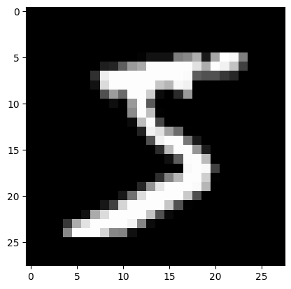
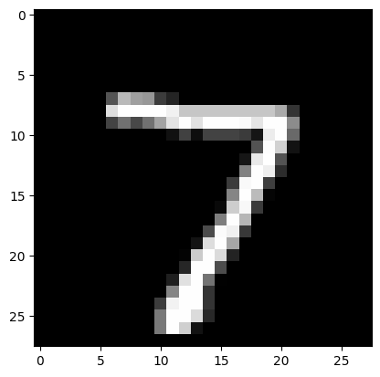
我们将使用众所周知的MNIST数据集,这是一组70,000张手写数字图像,我们将通过旋转图像在数据集上生成逐渐的分布变化。因此,最终的图将描绘随着旋转度的增加(x轴)预测分布(y轴)的熵的变化。上面的纸显示了一个图像的结果。另一方面,我们将对多个图像进行平均,以便在模型之间进行更好的比较。
我们将使用旋转来模拟平滑的移动。以下是旋转给定图像的方法:
[28]:
from PIL import Image
from torchvision import datasets
from torch.nn.functional import softmax
from torchvision.transforms.functional import rotate
[29]:
def imshow(image):
    plt.imshow(image, cmap='gray', vmin=0, vmax=255)
    plt.show()
[30]:
def show_rotation_on_mnist_example_image():
    mnist_train = datasets.MNIST('../data', train=True, download=True)
    image = Image.fromarray(mnist_train.data[0].numpy())
    imshow(image)
    rotated_image = rotate(image, angle=90)
    imshow(rotated_image)
[31]:
show_rotation_on_mnist_example_image()
Downloading http://yann.lecun.com/exdb/mnist/train-images-idx3-ubyte.gz
Downloading http://yann.lecun.com/exdb/mnist/train-images-idx3-ubyte.gz to ../data/MNIST/raw/train-images-idx3-ubyte.gz
100%|██████████| 9912422/9912422 [00:00<00:00, 104013908.09it/s]
Extracting ../data/MNIST/raw/train-images-idx3-ubyte.gz to ../data/MNIST/raw

Downloading http://yann.lecun.com/exdb/mnist/train-labels-idx1-ubyte.gz
Downloading http://yann.lecun.com/exdb/mnist/train-labels-idx1-ubyte.gz to ../data/MNIST/raw/train-labels-idx1-ubyte.gz
100%|██████████| 28881/28881 [00:00<00:00, 108837101.37it/s]
Extracting ../data/MNIST/raw/train-labels-idx1-ubyte.gz to ../data/MNIST/raw

Downloading http://yann.lecun.com/exdb/mnist/t10k-images-idx3-ubyte.gz
Downloading http://yann.lecun.com/exdb/mnist/t10k-images-idx3-ubyte.gz to ../data/MNIST/raw/t10k-images-idx3-ubyte.gz
100%|██████████| 1648877/1648877 [00:00<00:00, 25836124.81it/s]
Extracting ../data/MNIST/raw/t10k-images-idx3-ubyte.gz to ../data/MNIST/raw

Downloading http://yann.lecun.com/exdb/mnist/t10k-labels-idx1-ubyte.gz
Downloading http://yann.lecun.com/exdb/mnist/t10k-labels-idx1-ubyte.gz to ../data/MNIST/raw/t10k-labels-idx1-ubyte.gz
100%|██████████| 4542/4542 [00:00<00:00, 15024076.32it/s]
Extracting ../data/MNIST/raw/t10k-labels-idx1-ubyte.gz to ../data/MNIST/raw

让我们设置培训和测试数据:
[32]:
def get_mnist_data(train=True):
    mnist_data = datasets.MNIST('../data', train=train, download=True)
    x = mnist_data.data.reshape(-1, 28 * 28).float()
    y = mnist_data.targets
    return x, y

x_train, y_train = get_mnist_data(train=True)
x_test, y_test = get_mnist_data(train=False)
现在我们有了数据,让我们开始训练神经网络。
确定性网络
我们将使用不同的超参数重复使用我们的MLP网络架构:
[33]:
net = MLP(input_dim=784, output_dim=10, hidden_dim=30, n_hidden_layers=3)
培养
[34]:
def train_on_mnist(net):
    x_train, y_train = get_mnist_data(train=True)
    optimizer = torch.optim.Adam(params=net.parameters(), lr=1e-4)
    criterion = nn.CrossEntropyLoss()
    batch_size = 250

    progress_bar = trange(20)
    for _ in progress_bar:
        for batch_idx in range(int(x_train.shape[0] / batch_size)):
            batch_low, batch_high = batch_idx * batch_size, (batch_idx + 1) * batch_size
            optimizer.zero_grad()
            loss = criterion(target=y_train[batch_low:batch_high], input=net(x_train[batch_low:batch_high]))
            progress_bar.set_postfix(loss=f'{loss / batch_size:.3f}')
            loss.backward()
            optimizer.step()
    return net
[35]:
net = train_on_mnist(net)
试验
[36]:
def accuracy(targets, predictions):
  return (targets == predictions).sum() / targets.shape[0]
[37]:
def evaluate_accuracy_on_mnist(net):
    test_data = get_mnist_data(train=False)
    x_test, y_test = test_data
    net.eval()
    y_preds = net(x_test).argmax(1)
    acc = accuracy(y_test, y_preds)
    print("Test accuracy is %.2f%%" % (acc.item() * 100))
[38]:
evaluate_accuracy_on_mnist(net)
Test accuracy is 92.53%
旋转图像
现在让我们计算一些旋转图像的预测熵…
首先,我们将从测试图像中生成旋转角度不断增加的旋转图像。我们使用MNIST测试集的子集进行评估:
[39]:
def get_mnist_test_subset(n_test_images):
    mnist_test = datasets.MNIST('../data', train=False, download=True)
    x = mnist_test.data[:n_test_images].float()
    y = mnist_test.targets[:n_test_images]
    return x, y
[40]:
n_test_images = 100
x_test_subset, y_test_subset = get_mnist_test_subset(n_test_images=n_test_images)
[41]:
rotation_angles = [3 * i for i in range(0, 31)] # use angles from 0 to 90 degrees
rotated_images = [rotate(x_test_subset, angle).reshape(-1, 28 * 28) for angle in rotation_angles]
在旋转的图像上评估训练的MLP:
[42]:
y_preds_deterministic = [softmax(net(images), dim=-1) for images in rotated_images]
这信息熵 H概率分布的p一个离散的随机变量X可能的结果x1,…,xN,以概率发生p(xi):=pi由下式给出:
H(p)=−∑i=1Npi原木pi
熵在某种意义上量化了概率分布的不确定性,假设实验从分布中抽取的结果越不确定,熵就越高。最高是在所有可能的结果上平均分配概率质量。在我们的情况下,确定性神经网络估计每幅图像的MNIST上十个数字类别的概率分布。因此,对于旋转的图像,我们可以计算旋转角度上的熵。
1.1随着图像旋转角度的增加,您预计熵会如何表现?
1.2根据上面的公式实现计算熵的函数。
[43]:
def entropy(p):
  # return NotImplemented
  return (-p * np.log(p)).sum(axis=1)
现在,我们可以计算所有旋转图像的精度和熵,并绘制两者:
[44]:
def calculate_accuracies_and_entropies(y_preds):
    accuracies = [accuracy(y_test_subset, p.argmax(axis=1)) for p in y_preds]
    entropies = [np.mean(entropy(p.detach().numpy())) for p in y_preds]
    return accuracies, entropies
[45]:
def plot_accuracy_and_entropy(add_to_plot):
    fig, ax = plt.subplots(figsize=(10, 5))
    plt.xlim([0, 90])
    plt.xlabel("Rotation Angle", fontsize=20)

    add_to_plot(ax)

    plt.legend()
    plt.show()
[46]:
def add_deterministic(ax):
    accuracies, entropies = calculate_accuracies_and_entropies(y_preds_deterministic)
    ax.plot(rotation_angles, accuracies, 'b--', linewidth=3, label="Accuracy, Deterministic")
    ax.plot(rotation_angles, entropies, 'b-', linewidth=3, label="Entropy, Deterministic")
plot_accuracy_and_entropy(add_deterministic)

你对上面这个情节的解释是什么:预测熵在变化吗?如果是,你如何解释这一点?
蒙特卡洛辍学网络
让我们创建我们的辍学网络。为了公平的模型比较,我们保持网络深度和隐藏层大小与MLP相同
[47]:
net_dropout = MLP(input_dim=784, output_dim=10, hidden_dim=30, n_hidden_layers=3, use_dropout=True)
培养
[48]:
net_dropout = train_on_mnist(net_dropout)
试验
[49]:
evaluate_accuracy_on_mnist(net_dropout)
Test accuracy is 92.46%
评估旋转后的图像
2.1对100个不同的漏失屏蔽进行采样,并对其预测进行平均。
[50]:
n_dropout_samples = 100
net_dropout.train()  # we set the model to train to 'activate' the dropout layer

# y_preds_dropout = NotImplemented
y_preds_dropout = []
for image in rotated_images:
  y_preds = torch.zeros((n_test_images, 10))
  for idx in range(n_dropout_samples):
    y_preds += softmax(net_dropout(image), dim=1)
  y_preds_dropout.append(y_preds/n_dropout_samples)
2.2计算预测平均值的最佳方法是什么?您应该先计算网络输出的平均值,然后应用softmax,还是反过来?
[51]:
def add_deterministic_and_dropout(ax):
    accuracies, entropies = calculate_accuracies_and_entropies(y_preds_deterministic)
    ax.plot(rotation_angles, accuracies, 'b--', linewidth=3, label="Accuracy, Deterministic")
    ax.plot(rotation_angles, entropies, 'b-', linewidth=3, label="Entropy, Deterministic")

    accuracies, entropies = calculate_accuracies_and_entropies(y_preds_dropout)
    ax.plot(rotation_angles, accuracies, 'r--', linewidth=3, label="Accuracy, MC Dropout")
    ax.plot(rotation_angles, entropies, 'r-', linewidth=3, label="Entropy, MC Dropout")
plot_accuracy_and_entropy(add_deterministic_and_dropout)

MLP与MC-Dropout Network相比如何?(贝叶斯方法有什么好处吗?)
深度合奏
现在让我们来研究一下深层合奏的表现。我们将使用与MLP完全相同的网络超参数:
3.1使用上述相同的超参数定义和训练五个MLP的集合。
[52]:
ensemble_size = 5

# ensemble = NotImplemented
ensemble = []
for _ in range(ensemble_size):
  ensemble.append(MLP(input_dim=784, output_dim=10, hidden_dim=30, n_hidden_layers=3))
培养
[53]:
# ensemble = NotImplemented
for net in ensemble:
  train_on_mnist(net)
试验
3.2评估集合预报的准确性。你如何对集合成员给出的多个不同的预测进行最好的汇总?和上面的回归设置有什么区别?
[54]:
# y_preds = NotImplemented
y_preds = []
for net in ensemble:
  net.eval()
  y_preds.append(net(x_test).argmax(dim=1))
y_preds = torch.stack(y_preds, dim=0).to(torch.float)
y_preds = torch.mean(y_preds, dim=0)

acc = accuracy(y_test, y_preds)
print("Test accuracy is %.2f%%" % (acc.item() * 100))
Test accuracy is 84.61%
评估旋转后的图像
3.3再次计算预测值的平均值,但这次是全体成员的平均值。
[55]:
# y_preds_ensemble = NotImplemented
y_preds_ensemble = []
for image in rotated_images:
  y_preds = torch.zeros((n_test_images, 10))
  for net in ensemble:
    y_preds += softmax(net(image), dim=1)
  y_preds_ensemble.append(y_preds/ensemble_size)
[56]:
def add_deep_ensemble(ax):
    accuracies, entropies = calculate_accuracies_and_entropies(y_preds_deterministic)
    ax.plot(rotation_angles, accuracies, 'b--', linewidth=3, label="Accuracy, Deterministic")
    ax.plot(rotation_angles, entropies, 'b-', linewidth=3, label="Entropy, Deterministic")

    accuracies, entropies = calculate_accuracies_and_entropies(y_preds_dropout)
    ax.plot(rotation_angles, accuracies, 'r--', linewidth=3, label="Accuracy, MC Dropout")
    ax.plot(rotation_angles, entropies, 'r-', linewidth=3, label="Entropy, MC Dropout")

    accuracies, entropies = calculate_accuracies_and_entropies(y_preds_ensemble)
    ax.plot(rotation_angles, accuracies, 'g--', linewidth=3, label="Accuracy, Deep Ensemble")
    ax.plot(rotation_angles, entropies, 'g-', linewidth=3, label="Entropy, Deep Ensemble")
[57]:
plot_accuracy_and_entropy(add_deep_ensemble)
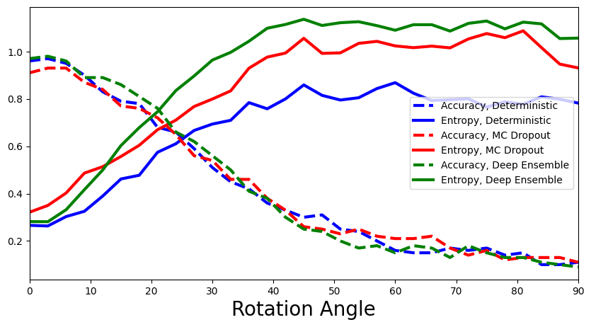
表演有什么不同吗?解释为什么你看到或没有看到任何差异。
贝叶斯神经网络
首先安装pyro包:
[58]:
!pip install pyro-ppl
Looking in indexes: https://pypi.org/simple, https://us-python.pkg.dev/colab-wheels/public/simple/
Collecting pyro-ppl
  Downloading pyro_ppl-1.8.4-py3-none-any.whl (730 kB)
     ━━━━━━━━━━━━━━━━━━━━━━━━━━━━━━━━━━━━━━ 730.7/730.7 kB 14.0 MB/s eta 0:00:00
Requirement already satisfied: numpy>=1.7 in /usr/local/lib/python3.9/dist-packages (from pyro-ppl) (1.22.4)
Collecting pyro-api>=0.1.1
  Downloading pyro_api-0.1.2-py3-none-any.whl (11 kB)
Requirement already satisfied: opt-einsum>=2.3.2 in /usr/local/lib/python3.9/dist-packages (from pyro-ppl) (3.3.0)
Requirement already satisfied: torch>=1.11.0 in /usr/local/lib/python3.9/dist-packages (from pyro-ppl) (2.0.0+cu118)
Requirement already satisfied: tqdm>=4.36 in /usr/local/lib/python3.9/dist-packages (from pyro-ppl) (4.65.0)
Requirement already satisfied: jinja2 in /usr/local/lib/python3.9/dist-packages (from torch>=1.11.0->pyro-ppl) (3.1.2)
Requirement already satisfied: networkx in /usr/local/lib/python3.9/dist-packages (from torch>=1.11.0->pyro-ppl) (3.1)
Requirement already satisfied: sympy in /usr/local/lib/python3.9/dist-packages (from torch>=1.11.0->pyro-ppl) (1.11.1)
Requirement already satisfied: filelock in /usr/local/lib/python3.9/dist-packages (from torch>=1.11.0->pyro-ppl) (3.11.0)
Requirement already satisfied: typing-extensions in /usr/local/lib/python3.9/dist-packages (from torch>=1.11.0->pyro-ppl) (4.5.0)
Requirement already satisfied: triton==2.0.0 in /usr/local/lib/python3.9/dist-packages (from torch>=1.11.0->pyro-ppl) (2.0.0)
Requirement already satisfied: cmake in /usr/local/lib/python3.9/dist-packages (from triton==2.0.0->torch>=1.11.0->pyro-ppl) (3.25.2)
Requirement already satisfied: lit in /usr/local/lib/python3.9/dist-packages (from triton==2.0.0->torch>=1.11.0->pyro-ppl) (16.0.1)
Requirement already satisfied: MarkupSafe>=2.0 in /usr/local/lib/python3.9/dist-packages (from jinja2->torch>=1.11.0->pyro-ppl) (2.1.2)
Requirement already satisfied: mpmath>=0.19 in /usr/local/lib/python3.9/dist-packages (from sympy->torch>=1.11.0->pyro-ppl) (1.3.0)
Installing collected packages: pyro-api, pyro-ppl
Successfully installed pyro-api-0.1.2 pyro-ppl-1.8.4
[59]:
import pyro
import pyro.distributions as dist
from pyro.nn import PyroModule, PyroSample
from pyro.infer import Predictive
from pyro.infer import SVI, Trace_ELBO
from pyro.infer.autoguide import AutoDiagonalNormal
from pyro.distributions import Normal, Categorical
from torch.nn.functional import softmax
from tqdm.auto import trange, tqdm
4.1实施用于分类MNIST数字的贝叶斯神经网络。对于定位,您可以使用第一个教程。
作为主干使用笔记本开头介绍的MLP架构。但是,因为我们将实现一个自定义指南(),明确定义每一层。
[60]:
class My_MLP(nn.Module):
  '''
  Implement a MLP with 3 hidden layers, Tanh activation, no dropout or residual connections
  '''
  def __init__(self, in_dim=784, out_dim=10, hid_dim=200):
    super().__init__()
    assert in_dim > 0
    assert out_dim > 0
    assert hid_dim > 0
    # activation
    # self.act =
    self.act = nn.Tanh()

    #3 hidden layers
    # self.fc1 =
    # self.fc2 =
    # self.fc3 =
    # self.out =
    # raise NotImplemented
    self.fc1 = nn.Linear(in_dim, hid_dim)
    self.fc2 = nn.Linear(hid_dim, hid_dim)
    self.fc3 = nn.Linear(hid_dim, hid_dim)
    self.out = nn.Linear(hid_dim, out_dim)

  def forward(self, x):
    # raise NotImplemented
    x = self.act(self.fc1(x))
    x = self.act(self.fc2(x))
    x = self.act(self.fc3(x))
    pred = self.out(x).squeeze()
    return pred
初始化网络。您必须在模型和向导函数中访问它的图层
[61]:
net = My_MLP()
[62]:
#confirm your layer names
for name, _ in net.named_parameters():
    print(name)
fc1.weight
fc1.bias
fc2.weight
fc2.bias
fc3.weight
fc3.bias
out.weight
out.bias
定义模型:> Pyro中的概率模型被指定为型号()功能。该函数定义了输出数据的生成方式。在model()函数中,首先是pyro模块随机模块()将神经网络的参数转换成具有先验概率分布的随机变量。第二,在pyro样品我们定义网络的输出是分类的,而pyro盘子允许我们向量化这个函数以提高计算效率。
提示:记住我们是在做分类而不是回归!
您可以“欺骗”一下:为了加快训练速度,并进一步限制我们需要优化的参数数量,实现一个BNN,其中只有最后一层是贝叶斯!
[63]:
def model(x_data, y_data):
  # raise NotImplemented
  outw_prior = Normal(loc=torch.zeros_like(net.out.weight), scale=torch.ones_like(net.out.weight)).to_event(2)
  outb_prior = Normal(loc=torch.zeros_like(net.out.bias), scale=torch.ones_like(net.out.bias)).to_event(1)
  priors = {'out.weight': outw_prior, 'out.bias': outb_prior}
  # lift module parameters to random variables sampled from the priors
  lifted_module = pyro.random_module("module", net, priors)
  # sample a regressor (which also samples w and b)
  lifted_reg_model = lifted_module()
  with pyro.plate("data", x_data.shape[0]):
        yhat = softmax(lifted_reg_model(x_data), dim=1)
        obs = pyro.sample("obs", dist.Categorical(yhat), obs=y_data)
实现指南(),变分分布: >该指南允许我们初始化一个性能良好的分布,稍后我们可以对其进行优化以逼近真实的后验概率
[64]:
softplus = torch.nn.Softplus()

def my_guide(x_data, y_data):
  # raise NotImplemented
  # Output layer weight distribution priors
  outw_mu_param = pyro.param("outw_mu", torch.randn_like(net.out.weight))
  outw_sigma_param = softplus(pyro.param("outw_sigma", torch.randn_like(net.out.weight)))
  outw_prior = Normal(loc=outw_mu_param, scale=outw_sigma_param).to_event(2)
  # Output layer bias distribution priors
  outb_mu_param = pyro.param("outb_mu", torch.randn_like(net.out.bias))
  outb_sigma_param = softplus(pyro.param("outb_sigma", torch.randn_like(net.out.bias)))
  outb_prior = Normal(loc=outb_mu_param, scale=outb_sigma_param).to_event(1)

  priors = {'out.weight': outw_prior, 'out.bias': outb_prior}
  lifted_module = pyro.random_module("module", net, priors)
  return lifted_module()
初始化随机变分推理(SVI)
[65]:
adam = pyro.optim.Adam({"lr": 1e-3})
# svi = raise NotImplemented
svi = SVI(model, my_guide, adam, loss=Trace_ELBO())
培养
[66]:
pyro.clear_param_store()
batch_size = 250
bar = trange(30)
for epoch in bar:
  for batch_idx in range(int(x_train.shape[0] / batch_size)):
    batch_low, batch_high = batch_idx * batch_size, (batch_idx+1) * batch_size
    loss = svi.step(x_train[batch_low:batch_high], y_train[batch_low:batch_high])
    bar.set_postfix(loss=f'{loss / batch_size:.3f}')
/usr/local/lib/python3.9/dist-packages/pyro/primitives.py:491: FutureWarning: The `random_module` primitive is deprecated, and will be removed in a future release. Use `pyro.nn.Module` to create Bayesian modules from `torch.nn.Module` instances.
  warnings.warn(
试验
使用学到的知识指南()函数来进行预测。为什么?因为型号()函数知道传道者对于权重和偏差,不博学的后验。这指南()包含参数值的近似后验分布,我们希望用它来进行预测。
[67]:
# y_preds = NotImplemented
num_samples = 10
def predict(x):
    sampled_models = [my_guide(None, None) for _ in range(num_samples)]
    yhats = [model(x).data for model in sampled_models]
    mean = torch.mean(torch.stack(yhats), 0)
    return mean
y_preds = predict(x_test).argmax(dim=1)


acc = accuracy(y_test, y_preds)
print("Test accuracy is %.2f%%" % (acc.item() * 100))
Test accuracy is 90.77%
评估旋转后的图像
[68]:
# y_preds_bnn = NotImplemented

num_samples = 50
def predict_probability(x):
    sampled_models = [my_guide(None, None) for _ in range(num_samples)]
    yhats = [softmax(model(x).data, dim=1) for model in sampled_models]
    mean = torch.mean(torch.stack(yhats), 0)
    return mean

y_preds_bnn = []
for image in rotated_images:
  y_preds_bnn.append(predict_probability(image))
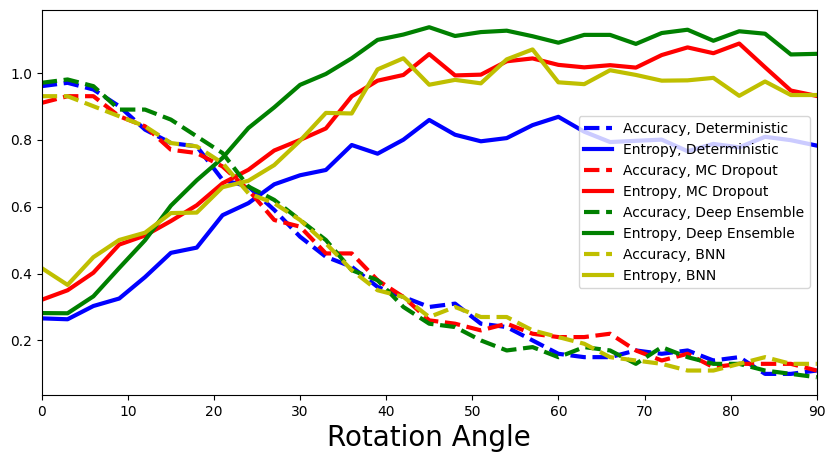
4.2显示所有四个模型的熵。哪种方法最适合检测分布偏移?你怎么解释这个?
[69]:
#add the computed values for BNN
def add_bnn(ax):
  # raise NotImplemented
  accuracies, entropies = calculate_accuracies_and_entropies(y_preds_deterministic)
  ax.plot(rotation_angles, accuracies, 'b--', linewidth=3, label="Accuracy, Deterministic")
  ax.plot(rotation_angles, entropies, 'b-', linewidth=3, label="Entropy, Deterministic")

  accuracies, entropies = calculate_accuracies_and_entropies(y_preds_dropout)
  ax.plot(rotation_angles, accuracies, 'r--', linewidth=3, label="Accuracy, MC Dropout")
  ax.plot(rotation_angles, entropies, 'r-', linewidth=3, label="Entropy, MC Dropout")

  accuracies, entropies = calculate_accuracies_and_entropies(y_preds_ensemble)
  ax.plot(rotation_angles, accuracies, 'g--', linewidth=3, label="Accuracy, Deep Ensemble")
  ax.plot(rotation_angles, entropies, 'g-', linewidth=3, label="Entropy, Deep Ensemble")

  accuracies, entropies = calculate_accuracies_and_entropies(y_preds_bnn)
  ax.plot(rotation_angles, accuracies, 'y--', linewidth=3, label="Accuracy, BNN")
  ax.plot(rotation_angles, entropies, 'y-', linewidth=3, label="Entropy, BNN")

plot_accuracy_and_entropy(add_bnn)
保形预测
在前面的模拟数据示例中,我们在回归任务的上下文中使用了保形预测。现在,我们正在看一个分类任务。虽然总体方案是相同的,但在具体的设计选择上有所不同。特别是,我们的模型输出现在是类别概率f^(x)∈[0,1]K,因此我们的预测集是离散集C^(Xn+1)⊆{1,…,K},在哪里K=10就MNIST而言。这与我们之前获得的连续不确定性带形成对比,并影响我们如何设计真实类和预测类的比较以获得我们的一致性分数.
因为保形预测通过预测集提供了不确定性的度量临时后即,在不改变模型训练过程的情况下,我们不能在通过熵检测分布偏移方面直接比较共形方法。相反,我们可以看看经验覆盖率和预测集大小。
5.1随着旋转角度的增加,您预计经验覆盖率和预测集大小会如何变化?
答:旋转角度越大,分布偏移越大,我们的校准数据为测试数据提供的信息就越少。这种分布不匹配应该反映在较低的实证覆盖率中。类似地,这种不匹配导致更高的预测不确定性,这应该反映在更大的预测集大小中。
培养
和前面的例子一样,我们将训练样本分成两个不同的数据集,真实训练集和校准集。我们从MNIST训练数据中取最后5k个样本作为校准样本。我们将前55k幅图像作为真实的训练样本。
[70]:
# split data into training and calibration sets

# raise NotImplemented
# x_cal, y_cal =
# x_tr, y_tr =

cal_idx = np.arange(55000, 60000, step=1, dtype=np.int64)
mask = np.zeros(60000, dtype=bool)
mask[cal_idx] = True
x_cal, y_cal = x_train[mask], y_train[mask]
x_tr, y_tr = x_train[~mask], y_train[~mask]
我们将在练习开始时重复使用确定性MLP网络架构,并在真实的训练集上对其进行训练:
[71]:
mlp = MLP(input_dim=784, output_dim=10, hidden_dim=30, n_hidden_layers=3)
[72]:
# training
mlp_optimizer = torch.optim.Adam(params=mlp.parameters(), lr=1e-4)
mlp_criterion = nn.CrossEntropyLoss()
batch_size = 250

bar = trange(30)
for epoch in bar:
  for batch_idx in range(int(x_train.shape[0] / batch_size)):
    batch_low, batch_high = batch_idx * batch_size, (batch_idx+1) * batch_size
    mlp_optimizer.zero_grad()
    loss = mlp_criterion(target=y_tr[batch_low:batch_high], input=mlp(x_tr[batch_low:batch_high]))
    bar.set_postfix(loss=f'{loss / batch_size:.3f}') #x.shape[0]
    loss.backward()
    mlp_optimizer.step()
试验
然后我们可以检查测试的准确性,以确保我们的模型训练良好。
[73]:
evaluate_accuracy_on_mnist(mlp)
Test accuracy is 93.09%
如果我们将精确度与根据完整数据训练的模型进行比较,我们可以得出什么结论?
分类设置的保形预测
如前所述,选择如何计算一致性分数是一个建模的决定。我们将看看最近文献中提出的三种不同的选择:
-
研究的朴素softmax方法Sadinle等人(2016年)
-
研究的自适应预测集(APS)方法罗马诺等人(2020年)
-
研究的正则化自适应预测集(RAPS)方法Angelopoulos等人(2021年)
为了便于介绍,建议阅读的第1章和第2章保形预测和无分布不确定性量化简介由Angelopoulos & Bates撰写,其中包含了针对我们的任务而改编的代码片段。
我们首先定义一些基本函数来计算保形分位数,以及平均预测大小和经验覆盖。
[74]:
def quantile(scores, alpha=0.1):
  # compute conformal quantile

  # raise NotImplemented
  # n =
  # q =
  # return np.quantile(...)

  n = len(scores)
  q_val = np.ceil((1 - alpha) * (n + 1)) / n
  return np.quantile(scores, q_val, method="higher")
[75]:
def mean_set_size(sets):
  # mean prediction set size
  return np.mean(np.sum(sets, axis=1), axis=0)
[76]:
def emp_coverage(sets, target):
  # empirical coverage
  return sets[np.arange(len(sets)), target].mean()
在这个方法中,我们定义了我们的一致性分数存在;成为si=1−π^xi(yi)对于一些校准样品(xi,yi),即一分钟真实(正确)类的softmax输出。我们对一些测试样本的预测集(xn+1,yn+1)然后被构造为C^(xn+1)={y′∈K:π^xn+1(y′)≥1−q^},即收集softmax分数高于阈值的所有类别1−q^。有关Imagenet的示例,请参见这里.
[77]:
# Calculate conformal quantile on calibration data
cal_smx = softmax(mlp(x_cal), dim=1).detach().numpy()
scores = 1 - cal_smx[np.arange(len(cal_idx)), y_cal.numpy()]
q = quantile(scores)
print(f"Softmax cut-off level: {1-q}")
Softmax cut-off level: 0.7470939755439758
[78]:
# Evaluate prediction sets on test data
test_smx = softmax(mlp(x_test), dim=1).detach().numpy()

# raise NotImplemented
# pred_sets =
pred_sets = test_smx >= (1-q)

print(f"Mean set size: {mean_set_size(pred_sets)}")
print(f"Empirical coverage: {emp_coverage(pred_sets, y_test.numpy())}")
Mean set size: 0.8977
Empirical coverage: 0.8726
经验覆盖率接近目标覆盖率90%,但没有完全达到目标覆盖率。也许不直观的是,平均集大小小于1。这是因为对于一些测试样本,构造的方法可以返回空集。如果没有softmax分数高于阈值,就会发生这种情况。虽然有排除空集的变通方法,但我们在这里不考虑它们。
对一些测试样本进行可视化…
[79]:
img_idx = 0 # compare e.g. img_idx = 4, 4000
plt.imshow(x_test[img_idx].reshape(28, 28), cmap='gray', vmin=0, vmax=255)
print(f"Prediction set: {pred_sets[img_idx].nonzero()[0].tolist()}")
Prediction set: [7]
现在让我们计算一些旋转MNIST图像的精确度、集合大小和经验覆盖率…
[80]:
deter_pred_means = []
for image in rotated_images:
  deter_pred_means.append(softmax(mlp(image), dim=1))
[81]:
acc = [accuracy(y_test[:n_test_images], p.argmax(axis=1)) for p in deter_pred_means]
set_size = [mean_set_size(p.detach().numpy() >= (1-q)) for p in deter_pred_means]
cov = [emp_coverage(p.detach().numpy() >= (1-q), y_test[:n_test_images].numpy()) for p in deter_pred_means]
[82]:
# generate plot

fig, ax = plt.subplots(figsize=(10, 5))
plt.xlim([0, 90])
plt.xlabel("Rotation Angle", fontsize=20)

ax.plot(rotation_angles, acc, 'b--', linewidth=3, label="Accuracy")
ax.plot(rotation_angles, set_size, 'b-', linewidth=3, label="Mean set size")
ax.plot(rotation_angles, cov, 'b:', linewidth=3, label="Emp. coverage")

plt.legend(loc=1, fontsize=15, frameon=False);
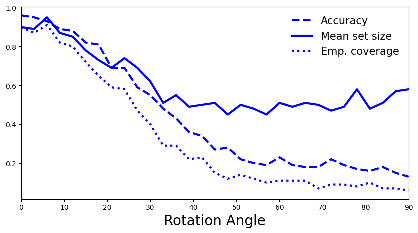
5.2你如何解读剧情?是你预料中的,还是有令人惊讶的趋势?如果是这样,你如何解释它?(提示:空集)
答:不出所料,随着旋转角度的增大,模型的精度下降,经验覆盖范围也减小。也许违反直觉的是,平均集大小也减少了。这是基于我们构建一致性分数的方式,特别是在计算𝑞̂时,我们只考虑正确类别的softmax分数。随着分布变化的增加,我们的模型的不确定性增加,这导致每个类别的softmax分数较低,因此阈值以上的分数较少。在这种意义上,更高的熵反映在更多的空集中,这降低了平均集大小。
在这个方法中,我们定义了我们的一致性分数存在;成为𝟙si=∑y′=1Kπ^xi(y′)1{π^xi(y′)>π^xi(y)}对于一些校准样品(xi,yi)。换句话说,我们将所有类别的softmax概率相加,直到达到真正的类别概率。与之前的方法相比,这允许我们不仅包含真实类的信息,还包含它与所有其他类的关系的信息,并且应该以整体更大的集合大小为代价,产生更自适应的预测集合。
某些测试样本的预测集(xn+1,yn+1)然后被构造为C^(xn+1)={y1,…,yk},在哪里k=小口喝;怎么了{k′:∑y′=1k′π^xn+1(y′)<q^}。换句话说,按大小对所有softmax分数进行排序,并将所有类包括在预测集中,直到它们的softmax分数之和达到q^。有关Imagenet的示例,请参见这里.
[83]:
# Calculate conformal quantile on calibration data
cal_smx = softmax(mlp(x_cal), dim=1).detach().numpy()
cal_pi = cal_smx.argsort(axis=1)[:, ::-1]
cal_srt = np.take_along_axis(cal_smx, cal_pi, axis=1).cumsum(axis=1)
scores = np.take_along_axis(cal_srt, cal_pi.argsort(axis=1), axis=1)[range(len(cal_idx)), y_cal.numpy()]
q = quantile(scores)
print(f"Softmax cut-off level: {q}")
Softmax cut-off level: 0.998565137386322
[84]:
# Evaluate prediction sets on test data
test_smx = softmax(mlp(x_test), dim=1).detach().numpy()
test_pi = test_smx.argsort(axis=1)[:, ::-1]
test_srt = np.take_along_axis(test_smx, test_pi, axis=1).cumsum(axis=1)

# raise NotImplemented
# pred_sets = np.take_along_axis(..., test_pi.argsort(axis=1), axis=1)
pred_sets = np.take_along_axis(test_srt <= q, test_pi.argsort(axis=1), axis=1)

print(f"Mean set size: {mean_set_size(pred_sets)}")
print(f"Empirical coverage: {emp_coverage(pred_sets, y_test.numpy())}")
Mean set size: 3.1416
Empirical coverage: 0.9157
对一些测试样本进行可视化…
[85]:
img_idx = 0 # compare e.g. img_idx = 4, 4000
plt.imshow(x_test[img_idx].reshape(28, 28), cmap='gray', vmin=0, vmax=255)
print(f"Prediction set: {pred_sets[img_idx].nonzero()[0].tolist()}")
Prediction set: []

现在让我们计算一些旋转MNIST图像的精确度、集合大小和经验覆盖率…
[86]:
deter_pred_means = []
for image in rotated_images:
  deter_pred_means.append(softmax(mlp(image), dim=1))
[87]:
acc = [accuracy(y_test[:n_test_images], p.argmax(axis=1)) for p in deter_pred_means]
[88]:
set_size, cov = [], []
for p in deter_pred_means:
  p = p.detach().numpy()
  p_pi = p.argsort(axis=1)[:, ::-1]
  p_srt = np.take_along_axis(p, p_pi, axis=1).cumsum(axis=1)
  pred_sets = np.take_along_axis(p_srt <= q, p_pi.argsort(axis=1), axis=1)
  set_size.append(mean_set_size(pred_sets))
  cov.append(emp_coverage(pred_sets, y_test[:n_test_images].numpy()))
[89]:
# generate plot

fig, ax = plt.subplots(figsize=(10, 5))
plt.xlim([0, 90])
plt.xlabel("Rotation Angle", fontsize=20)

ax.plot(rotation_angles, acc, 'b--', linewidth=3, label="Accuracy")
ax.plot(rotation_angles, set_size, 'b-', linewidth=3, label="Mean set size")
ax.plot(rotation_angles, cov, 'b:', linewidth=3, label="Emp. coverage")

plt.legend(loc=2, fontsize=15, frameon=False);

5.3你如何解读剧情?这是你所期望的吗?
答:正如预期的那样,随着旋转角度的增加,模型的准确性下降,其经验覆盖范围也下降,尽管速度比以前低。通过考虑一致性分数分位数q^在某种程度上更能适应变化。我们还观察了预测集大小的预期趋势。随着变化的增加,更高的预测不确定性反映在更大的集合大小中。请注意,对于我们只有10个类的任务来说,一个6+大小的集合在高轮班时变得非常没有意义。
该方法建立在APS的基础上,提出了一个额外的正则项来减少预测集的大小,同时保持保形覆盖保证。这引入了额外的参数,但大大减少了集合大小,使其在实践中更有用。正则项实质上增加了概率质量作为“惩罚”项λreg达到定义的阈值后的所有softmax分数kreg以更快地达到APS softmax阈值,从而产生更小的预测集。一般分数构造和APS差不多。为了进一步阅读,你可以看看这篇论文(第2.1和2.2节,也见图3)。有关Imagenet的示例,请参见这里.
[90]:
# Set RAPS regularization parameters
smx_classes = 10

lam_reg = 0.01 # Effect?
k_reg = 3 # Effect?

disallow_zero_sets = False # Set this to False in order to see the coverage upper bound hold
rand = True # Set this to True in order to see the coverage upper bound hold
reg_vec = np.array(k_reg * [0,] + (smx_classes - k_reg) * [lam_reg,])[None, :]
print(f"Probability mass penalty for each class: {reg_vec}")
Probability mass penalty for each class: [[0. 0. 0. 0.01 0.01 0.01 0.01 0.01 0.01 0.01]]
5.4尝试不同的参数设置。math:`lambda_{reg} '和math:`k_{reg} '对正则化有什么影响?
甲:大一点λreg通过施加更高的惩罚质量导致更小的集合,因此截止q^更快地到达。较小的kreg通过允许更多的类被扣分,导致更小的集合,导致更大的累积分数,再次达到截止值q^更快。
[91]:
# Calculate conformal quantile on calibration data
cal_smx = softmax(mlp(x_cal), dim=1).detach().numpy()

cal_pi = cal_smx.argsort(axis=1)[:, ::-1]
cal_srt = np.take_along_axis(cal_smx, cal_pi, axis=1)
cal_srt_reg = cal_srt + reg_vec
cal_L = np.where(cal_pi == y_cal.numpy()[:, None])[1]
n = len(cal_idx)

scores = cal_srt_reg.cumsum(axis=1)[np.arange(n), cal_L] - np.random.rand(n) * cal_srt_reg[np.arange(n), cal_L]
q = quantile(scores)
print(f"Softmax cut-off level: {q}")
Softmax cut-off level: 0.9008058661638462
[92]:
# Evaluate prediction sets on test data
test_smx = softmax(mlp(x_test), dim=1).detach().numpy()

test_pi = test_smx.argsort(1)[:, ::-1]
test_srt = np.take_along_axis(test_smx, test_pi, axis=1)
test_srt_reg = test_srt + reg_vec
test_srt_reg_cumsum = test_srt_reg.cumsum(axis=1)

if rand:
  indicators = (test_srt_reg.cumsum(axis=1) - np.random.rand(len(test_smx), 1) * test_srt_reg) <= q
else:
  indicators = (test_srt_reg.cumsum(axis=1) - test_srt_reg) <= q

if disallow_zero_sets:
  indicators[:, 0] = True

pred_sets = np.take_along_axis(indicators, test_pi.argsort(axis=1), axis=1)
print(f"Mean set size: {mean_set_size(pred_sets)}")
print(f"Empirical coverage: {emp_coverage(pred_sets, y_test.numpy())}")
Mean set size: 1.1334
Empirical coverage: 0.9051
这些指标与使用APS获得的未经调整的指标相比如何?
对一些测试样本进行可视化…
[93]:
img_idx = 0 # compare e.g. img_idx = 4, 4000
plt.imshow(x_test[img_idx].reshape(28, 28), cmap='gray', vmin=0, vmax=255)
print(f"Prediction set: {pred_sets[img_idx].nonzero()[0].tolist()}")
Prediction set: [7]

现在让我们计算一些旋转MNIST图像的精确度、集合大小和经验覆盖率…
[94]:
deter_pred_means = []
for image in rotated_images:
  deter_pred_means.append(softmax(mlp(image), dim=1))
[95]:
acc = [accuracy(y_test[:n_test_images], p.argmax(axis=1)) for p in deter_pred_means]
[96]:
set_size, cov = [], []
for p in deter_pred_means:
  p = p.detach().numpy()
  p_pi = p.argsort(1)[:, ::-1]
  p_srt = np.take_along_axis(p, p_pi, axis=1)
  p_srt_reg = p_srt + reg_vec
  p_srt_reg_cumsum = p_srt_reg.cumsum(axis=1)

  if rand:
    indicators = (p_srt_reg.cumsum(axis=1) - np.random.rand(len(p), 1) * p_srt_reg) <= q
  else:
    indicators = (p_srt_reg.cumsum(axis=1) - p_srt_reg) <= q

  if disallow_zero_sets:
    indicators[:, 0] = True

  pred_sets = np.take_along_axis(indicators, p_pi.argsort(axis=1), axis=1)
  set_size.append(mean_set_size(pred_sets))
  cov.append(emp_coverage(pred_sets, y_test[:n_test_images].numpy()))
[97]:
# generate plot

fig, ax = plt.subplots(figsize=(10, 5))
plt.xlim([0, 90])
plt.xlabel("Rotation Angle", fontsize=20)

ax.plot(rotation_angles, acc, 'b--', linewidth=3, label="Accuracy")
ax.plot(rotation_angles, set_size, 'b-', linewidth=3, label="Mean set size")
ax.plot(rotation_angles, cov, 'b:', linewidth=3, label="Emp. coverage")

plt.legend(loc=2, fontsize=15, frameon=False);

5.5你如何解读剧情?这是你所期望的吗?和没有正规化的APS相比如何?
答:我们再次观察到与AP相同的模式:更大的分布变化反映在准确性和经验覆盖范围的降低,以及预测集大小的增加。
5.6你得出什么结论?适形预测能够识别旋转MNIST图像引起的分布偏移吗?
答:我们的结论是,与目前提出的(近似)贝叶斯不确定性量化方法相比,共形预测方法也能够识别分布偏移,同时依赖非常不同的技术和度量。
版权所有2022,菲利普·利皮。修订本a8981a95.
阅读文件v:最新的


 1787
1787

 被折叠的 条评论
为什么被折叠?
被折叠的 条评论
为什么被折叠?
 到【灌水乐园】发言


