


脑电数据处理过程中如何去除伪迹是很重要的一个步骤,伪迹的处理主要包括眼电、心电、肌肉点以及工频干扰。实际处理过程中通过滤波0.5-45赫兹的带通滤波器可以去除掉大部分的噪音,在我接触到的实际脑电数数据中心电的伪迹大多数还真不是很明显,去伪迹的时候眼电的伪迹相对更加明显一些。MNE库中也有很多去伪迹的方法,这里给大家介绍一种ICA的方式。查看了一些文章,ICA在脑电数据处理中应用的也比较普遍。

采用ICA的方式去除伪迹,主要的工作就是分辨出ICA成分中的伪迹,实际上在你做完ICA后如果伪迹明显,还是很容易看出来的。在MNE提供的例子中默认你是有眼电心电记录的,通过ICA后的主成分和记录伪迹的相关性来判断伪迹。但是在实际的处理过程中,有可能你没有伪迹的记录,如何判断伪迹成分呢?
不同类型的伪迹有着一定的特点:
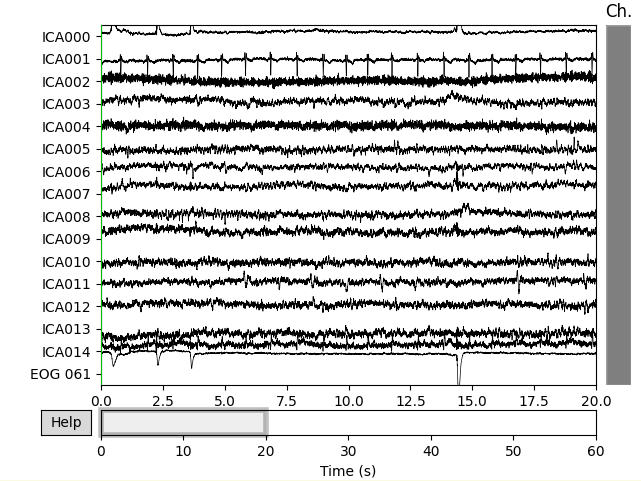
MNE中的例子:就算没有心电眼电的记录也基本能断定这里ICA000是眼电,ICA001是心电,你再和EOG061记录对比下,虽然幅值是反的,但形态基本一致。额外说一下如果是我处理的话,ICA002和ICA004也会去除,我认为这两个是干扰的噪声成分,可能是肌肉电也可能是噪声干扰,虽然滤波可以去除部分的频段,但难免有些噪声的频段是和脑电重合的啊。。。
实际的数据:红色圈出的我认为是眼电的伪迹
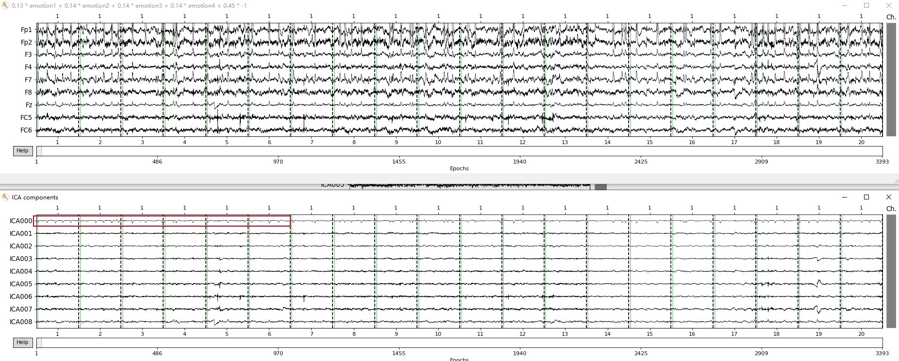
上面红色圈出部分的特写:眼电也就长这样了吧,呵呵。

MNE中提供的源码:改天写个这个代码的说明吧。
# -*- coding: utf-8 -*-
"""
.. _tut-artifact-ica:

Repairing artifacts with ICA
============================

This tutorial covers the basics of independent components analysis (ICA) and
shows how ICA can be used for artifact repair; an extended example illustrates
repair of ocular and heartbeat artifacts.

.. contents:: Page contents
   :local:
   :depth: 2

We begin as always by importing the necessary Python modules and loading some
:ref:`example data <sample-dataset>`. Because ICA can be computationally
intense, we'll also crop the data to 60 seconds; and to save ourselves from
repeatedly typing ``mne.preprocessing`` we'll directly import a few functions
and classes from that submodule:
"""


import os
import mne
from mne.preprocessing import (ICA, create_eog_epochs, create_ecg_epochs,
                               corrmap)

sample_data_folder = mne.datasets.sample.data_path()
sample_data_raw_file = os.path.join(sample_data_folder, 'MEG', 'sample',
                                    'sample_audvis_raw.fif')
raw = mne.io.read_raw_fif(sample_data_raw_file)
raw.crop(tmax=60.)

###############################################################################
# .. note::
#     Before applying ICA (or any artifact repair strategy), be sure to observe
#     the artifacts in your data to make sure you choose the right repair tool.
#     Sometimes the right tool is no tool at all — if the artifacts are small
#     enough you may not even need to repair them to get good analysis results.
#     See :ref:`tut-artifact-overview` for guidance on detecting and
#     visualizing various types of artifact.
#
# What is ICA?
# ^^^^^^^^^^^^
#
# Independent components analysis (ICA) is a technique for estimating
# independent source signals from a set of recordings in which the source
# signals were mixed together in unknown ratios. A common example of this is
# the problem of `blind source separation`_: with 3 musical instruments playing
# in the same room, and 3 microphones recording the performance (each picking
# up all 3 instruments, but at varying levels), can you somehow "unmix" the
# signals recorded by the 3 microphones so that you end up with a separate
# "recording" isolating the sound of each instrument?
#
# It is not hard to see how this analogy applies to EEG/MEG analysis: there are
# many "microphones" (sensor channels) simultaneously recording many
# "instruments" (blinks, heartbeats, activity in different areas of the brain,
# muscular activity from jaw clenching or swallowing, etc). As long as these
# various source signals are `statistically independent`_ and non-gaussian, it
# is usually possible to separate the sources using ICA, and then re-construct
# the sensor signals after excluding the sources that are unwanted.
#
#
# ICA in MNE-Python
# ~~~~~~~~~~~~~~~~~
#
# .. sidebar:: ICA and dimensionality reduction
#
#     If you want to perform ICA with *no* dimensionality reduction (other than
#     the number of Independent Components (ICs) given in ``n_components``, and
#     any subsequent exclusion of ICs you specify in ``ICA.exclude``), pass
#     ``max_pca_components=None`` and ``n_pca_components=None`` (these are the
#     default values).
#
#     However, if you *do* want to reduce dimensionality, consider this
#     example: if you have 300 sensor channels and you set
#     ``max_pca_components=200``, ``n_components=50`` and
#     ``n_pca_components=None``, then the PCA step yields 200 PCs, the first 50
#     PCs are sent to the ICA algorithm (yielding 50 ICs), and during
#     reconstruction :meth:`~mne.preprocessing.ICA.apply` will use the 50 ICs
#     plus PCs number 51-200 (the full PCA residual). If instead you specify
#     ``n_pca_components=120`` then :meth:`~mne.preprocessing.ICA.apply` will
#     reconstruct using the 50 ICs plus the first 70 PCs in the PCA residual
#     (numbers 51-120).
#
#     **If you have previously been using EEGLAB**'s ``runica()`` and are
#     looking for the equivalent of its ``'pca', n`` option to reduce
#     dimensionality via PCA before the ICA step, set ``max_pca_components=n``,
#     while leaving ``n_components`` and ``n_pca_components`` at their default
#     (i.e., ``None``).
#
# MNE-Python implements three different ICA algorithms: ``fastica`` (the
# default), ``picard``, and ``infomax``. FastICA and Infomax are both in fairly
# widespread use; Picard is a newer (2017) algorithm that is expected to
# converge faster than FastICA and Infomax, and is more robust than other
# algorithms in cases where the sources are not completely independent, which
# typically happens with real EEG/MEG data. See [1]_ for more information.
#
# The ICA interface in MNE-Python is similar to the interface in
# `scikit-learn`_: some general parameters are specified when creating an
# :class:`~mne.preprocessing.ICA` object, then the
# :class:`~mne.preprocessing.ICA` object is fit to the data using its
# :meth:`~mne.preprocessing.ICA.fit` method. The results of the fitting are
# added to the :class:`~mne.preprocessing.ICA` object as attributes that end in
# an underscore (``_``), such as ``ica.mixing_matrix_`` and
# ``ica.unmixing_matrix_``. After fitting, the ICA component(s) that you want
# to remove must be chosen, and the ICA fit must then be applied to the
# :class:`~mne.io.Raw` or :class:`~mne.Epochs` object using the
# :class:`~mne.preprocessing.ICA` object's :meth:`~mne.preprocessing.ICA.apply`
# method.
#
# As is typically done with ICA, the data are first scaled to unit variance and
# whitened using principal components analysis (PCA) before performing the ICA
# decomposition. You can impose an optional dimensionality reduction at this
# step by specifying ``max_pca_components``. From the retained Principal
# Components (PCs), the first ``n_components`` are then passed to the ICA
# algorithm (``n_components`` may be an integer number of components to use, or
# a fraction of explained variance that used components should capture).
#
# After visualizing the Independent Components (ICs) and excluding any that
# capture artifacts you want to repair, the sensor signal can be reconstructed
# using the :class:`~mne.preprocessing.ICA` object's
# :meth:`~mne.preprocessing.ICA.apply` method. By default, signal
# reconstruction uses all of the ICs (less any ICs listed in ``ICA.exclude``)
# plus all of the PCs that were not included in the ICA decomposition (i.e.,
# the "PCA residual"). If you want to reduce the number of components used at
# the reconstruction stage, it is controlled by the ``n_pca_components``
# parameter (which will in turn reduce the rank of your data; by default
# ``n_pca_components = max_pca_components`` resulting in no additional
# dimensionality reduction). The fitting and reconstruction procedures and the
# parameters that control dimensionality at various stages are summarized in
# the diagram below:
#
# .. graphviz:: ../../_static/diagrams/ica.dot
#    :alt: Diagram of ICA procedure in MNE-Python
#    :align: left
#
# See the Notes section of the :class:`~mne.preprocessing.ICA` documentation
# for further details. Next we'll walk through an extended example that
# illustrates each of these steps in greater detail.
#
# Example: EOG and ECG artifact repair
# ^^^^^^^^^^^^^^^^^^^^^^^^^^^^^^^^^^^^
#
# Visualizing the artifacts
# ~~~~~~~~~~~~~~~~~~~~~~~~~
#
# Let's begin by visualizing the artifacts that we want to repair. In this
# dataset they are big enough to see easily in the raw data:

# pick some channels that clearly show heartbeats and blinks
regexp = r'(MEG [12][45][123]1|EEG 00.)'
artifact_picks = mne.pick_channels_regexp(raw.ch_names, regexp=regexp)
raw.plot(order=artifact_picks, n_channels=len(artifact_picks))

###############################################################################
# We can get a summary of how the ocular artifact manifests across each channel
# type using :func:`~mne.preprocessing.create_eog_epochs` like we did in the
# :ref:`tut-artifact-overview` tutorial:

eog_evoked = create_eog_epochs(raw).average()
eog_evoked.apply_baseline(baseline=(None, -0.2))
eog_evoked.plot_joint()

###############################################################################
# Now we'll do the same for the heartbeat artifacts, using
# :func:`~mne.preprocessing.create_ecg_epochs`:

ecg_evoked = create_ecg_epochs(raw).average()
ecg_evoked.apply_baseline(baseline=(None, -0.2))
ecg_evoked.plot_joint()

###############################################################################
# Filtering to remove slow drifts
# ~~~~~~~~~~~~~~~~~~~~~~~~~~~~~~~
#
# Before we run the ICA, an important step is filtering the data to remove
# low-frequency drifts, which can negatively affect the quality of the ICA fit.
# The slow drifts are problematic because they reduce the independence of the
# assumed-to-be-independent sources (e.g., during a slow upward drift, the
# neural, heartbeat, blink, and other muscular sources will all tend to have
# higher values), making it harder for the algorithm to find an accurate
# solution. A high-pass filter with 1 Hz cutoff frequency is recommended.
# However, because filtering is a linear operation, the ICA solution found from
# the filtered signal can be applied to the unfiltered signal (see [2]_ for
# more information), so we'll keep a copy of the unfiltered
# :class:`~mne.io.Raw` object around so we can apply the ICA solution to it
# later.

filt_raw = raw.copy()
filt_raw.load_data().filter(l_freq=1., h_freq=None)

###############################################################################
# Fitting and plotting the ICA solution
# ~~~~~~~~~~~~~~~~~~~~~~~~~~~~~~~~~~~~~
#
# .. sidebar:: Ignoring the time domain
#
#     The ICA algorithms implemented in MNE-Python find patterns across
#     channels, but ignore the time domain. This means you can compute ICA on
#     discontinuous :class:`~mne.Epochs` or :class:`~mne.Evoked` objects (not
#     just continuous :class:`~mne.io.Raw` objects), or only use every Nth
#     sample by passing the ``decim`` parameter to ``ICA.fit()``.
#
# Now we're ready to set up and fit the ICA. Since we know (from observing our
# raw data) that the EOG and ECG artifacts are fairly strong, we would expect
# those artifacts to be captured in the first few dimensions of the PCA
# decomposition that happens before the ICA. Therefore, we probably don't need
# a huge number of components to do a good job of isolating our artifacts
# (though it is usually preferable to include more components for a more
# accurate solution). As a first guess, we'll run ICA with ``n_components=15``
# (use only the first 15 PCA components to compute the ICA decomposition) — a
# very small number given that our data has over 300 channels, but with the
# advantage that it will run quickly and we will able to tell easily whether it
# worked or not (because we already know what the EOG / ECG artifacts should
# look like).
#
# ICA fitting is not deterministic (e.g., the components may get a sign
# flip on different runs, or may not always be returned in the same order), so
# we'll also specify a `random seed`_ so that we get identical results each
# time this tutorial is built by our web servers.

ica = ICA(n_components=15, random_state=97)
ica.fit(filt_raw)

###############################################################################
# Some optional parameters that we could have passed to the
# :meth:`~mne.preprocessing.ICA.fit` method include ``decim`` (to use only
# every Nth sample in computing the ICs, which can yield a considerable
# speed-up) and ``reject`` (for providing a rejection dictionary for maximum
# acceptable peak-to-peak amplitudes for each channel type, just like we used
# when creating epoched data in the :ref:`tut-overview` tutorial).
#
# Now we can examine the ICs to see what they captured.
# :meth:`~mne.preprocessing.ICA.plot_sources` will show the time series of the
# ICs. Note that in our call to :meth:`~mne.preprocessing.ICA.plot_sources` we
# can use the original, unfiltered :class:`~mne.io.Raw` object:

raw.load_data()
ica.plot_sources(raw)

###############################################################################
# Here we can pretty clearly see that the first component (``ICA000``) captures
# the EOG signal quite well, and the second component (``ICA001``) looks a lot
# like `a heartbeat <qrs_>`_ (for more info on visually identifying Independent
# Components, `this EEGLAB tutorial`_ is a good resource). We can also
# visualize the scalp field distribution of each component using
# :meth:`~mne.preprocessing.ICA.plot_components`. These are interpolated based
# on the values in the ICA unmixing matrix:

# sphinx_gallery_thumbnail_number = 9
ica.plot_components()

###############################################################################
# .. note::
#
#     :meth:`~mne.preprocessing.ICA.plot_components` (which plots the scalp
#     field topographies for each component) has an optional ``inst`` parameter
#     that takes an instance of :class:`~mne.io.Raw` or :class:`~mne.Epochs`.
#     Passing ``inst`` makes the scalp topographies interactive: clicking one
#     will bring up a diagnostic :meth:`~mne.preprocessing.ICA.plot_properties`
#     window (see below) for that component.
#
# In the plots above it's fairly obvious which ICs are capturing our EOG and
# ECG artifacts, but there are additional ways visualize them anyway just to
# be sure. First, we can plot an overlay of the original signal against the
# reconstructed signal with the artifactual ICs excluded, using
# :meth:`~mne.preprocessing.ICA.plot_overlay`:

# blinks
ica.plot_overlay(raw, exclude=[0], picks='eeg')
# heartbeats
ica.plot_overlay(raw, exclude=[1], picks='mag')

###############################################################################
# We can also plot some diagnostics of each IC using
# :meth:`~mne.preprocessing.ICA.plot_properties`:

ica.plot_properties(raw, picks=[0, 1])

###############################################################################
# In the remaining sections, we'll look at different ways of choosing which ICs
# to exclude prior to reconstructing the sensor signals.
#
#
# Selecting ICA components manually
# ~~~~~~~~~~~~~~~~~~~~~~~~~~~~~~~~~
#
# Once we're certain which components we want to exclude, we can specify that
# manually by setting the ``ica.exclude`` attribute. Similar to marking bad
# channels, merely setting ``ica.exclude`` doesn't do anything immediately (it
# just adds the excluded ICs to a list that will get used later when it's
# needed). Once the exclusions have been set, ICA methods like
# :meth:`~mne.preprocessing.ICA.plot_overlay` will exclude those component(s)
# even if no ``exclude`` parameter is passed, and the list of excluded
# components will be preserved when using :meth:`mne.preprocessing.ICA.save`
# and :func:`mne.preprocessing.read_ica`.

ica.exclude = [0, 1]  # indices chosen based on various plots above

###############################################################################
# Now that the exclusions have been set, we can reconstruct the sensor signals
# with artifacts removed using the :meth:`~mne.preprocessing.ICA.apply` method
# (remember, we're applying the ICA solution from the *filtered* data to the
# original *unfiltered* signal). Plotting the original raw data alongside the
# reconstructed data shows that the heartbeat and blink artifacts are repaired.

# ica.apply() changes the Raw object in-place, so let's make a copy first:
reconst_raw = raw.copy()
ica.apply(reconst_raw)

raw.plot(order=artifact_picks, n_channels=len(artifact_picks))
reconst_raw.plot(order=artifact_picks, n_channels=len(artifact_picks))
del reconst_raw

###############################################################################
# Using an EOG channel to select ICA components
# ~~~~~~~~~~~~~~~~~~~~~~~~~~~~~~~~~~~~~~~~~~~~~
#
# It may have seemed easy to review the plots and manually select which ICs to
# exclude, but when processing dozens or hundreds of subjects this can become
# a tedious, rate-limiting step in the analysis pipeline. One alternative is to
# use dedicated EOG or ECG sensors as a "pattern" to check the ICs against, and
# automatically mark for exclusion any ICs that match the EOG/ECG pattern. Here
# we'll use :meth:`~mne.preprocessing.ICA.find_bads_eog` to automatically find
# the ICs that best match the EOG signal, then use
# :meth:`~mne.preprocessing.ICA.plot_scores` along with our other plotting
# functions to see which ICs it picked. We'll start by resetting
# ``ica.exclude`` back to an empty list:

ica.exclude = []
# find which ICs match the EOG pattern
eog_indices, eog_scores = ica.find_bads_eog(raw)
ica.exclude = eog_indices

# barplot of ICA component "EOG match" scores
ica.plot_scores(eog_scores)

# plot diagnostics
ica.plot_properties(raw, picks=eog_indices)

# plot ICs applied to raw data, with EOG matches highlighted
ica.plot_sources(raw)

# plot ICs applied to the averaged EOG epochs, with EOG matches highlighted
ica.plot_sources(eog_evoked)

###############################################################################
# Note that above we used :meth:`~mne.preprocessing.ICA.plot_sources` on both
# the original :class:`~mne.io.Raw` instance and also on an
# :class:`~mne.Evoked` instance of the extracted EOG artifacts. This can be
# another way to confirm that :meth:`~mne.preprocessing.ICA.find_bads_eog` has
# identified the correct components.
#
#
# Using a simulated channel to select ICA components
# ~~~~~~~~~~~~~~~~~~~~~~~~~~~~~~~~~~~~~~~~~~~~~~~~~~
#
# If you don't have an EOG channel,
# :meth:`~mne.preprocessing.ICA.find_bads_eog` has a ``ch_name`` parameter that
# you can use as a proxy for EOG. You can use a single channel, or create a
# bipolar reference from frontal EEG sensors and use that as virtual EOG
# channel. This carries a risk however: you must hope that the frontal EEG
# channels only reflect EOG and not brain dynamics in the prefrontal cortex (or
# you must not care about those prefrontal signals).
#
# For ECG, it is easier: :meth:`~mne.preprocessing.ICA.find_bads_ecg` can use
# cross-channel averaging of magnetometer or gradiometer channels to construct
# a virtual ECG channel, so if you have MEG channels it is usually not
# necessary to pass a specific channel name.
# :meth:`~mne.preprocessing.ICA.find_bads_ecg` also has two options for its
# ``method`` parameter: ``'ctps'`` (cross-trial phase statistics [3]_) and
# ``'correlation'`` (Pearson correlation between data and ECG channel).

ica.exclude = []
# find which ICs match the ECG pattern
ecg_indices, ecg_scores = ica.find_bads_ecg(raw, method='correlation')
ica.exclude = ecg_indices

# barplot of ICA component "ECG match" scores
ica.plot_scores(ecg_scores)

# plot diagnostics
ica.plot_properties(raw, picks=ecg_indices)

# plot ICs applied to raw data, with ECG matches highlighted
ica.plot_sources(raw)

# plot ICs applied to the averaged ECG epochs, with ECG matches highlighted
ica.plot_sources(ecg_evoked)

###############################################################################
# The last of these plots is especially useful: it shows us that the heartbeat
# artifact is coming through on *two* ICs, and we've only caught one of them.
# In fact, if we look closely at the output of
# :meth:`~mne.preprocessing.ICA.plot_sources` (online, you can right-click →
# "view image" to zoom in), it looks like ``ICA014`` has a weak periodic
# component that is in-phase with ``ICA001``. It might be worthwhile to re-run
# the ICA with more components to see if that second heartbeat artifact
# resolves out a little better:

# refit the ICA with 30 components this time
new_ica = ICA(n_components=30, random_state=97)
new_ica.fit(filt_raw)

# find which ICs match the ECG pattern
ecg_indices, ecg_scores = new_ica.find_bads_ecg(raw, method='correlation')
new_ica.exclude = ecg_indices

# barplot of ICA component "ECG match" scores
new_ica.plot_scores(ecg_scores)

# plot diagnostics
new_ica.plot_properties(raw, picks=ecg_indices)

# plot ICs applied to raw data, with ECG matches highlighted
new_ica.plot_sources(raw)

# plot ICs applied to the averaged ECG epochs, with ECG matches highlighted
new_ica.plot_sources(ecg_evoked)

###############################################################################
# Much better! Now we've captured both ICs that are reflecting the heartbeat
# artifact (and as a result, we got two diagnostic plots: one for each IC that
# reflects the heartbeat). This demonstrates the value of checking the results
# of automated approaches like :meth:`~mne.preprocessing.ICA.find_bads_ecg`
# before accepting them.

# clean up memory before moving on
del raw, filt_raw, ica, new_ica

###############################################################################
# Selecting ICA components using template matching
# ~~~~~~~~~~~~~~~~~~~~~~~~~~~~~~~~~~~~~~~~~~~~~~~~
#
# When dealing with multiple subjects, it is also possible to manually select
# an IC for exclusion on one subject, and then use that component as a
# *template* for selecting which ICs to exclude from other subjects' data,
# using :func:`mne.preprocessing.corrmap` [4]_. The idea behind
# :func:`~mne.preprocessing.corrmap` is that the artifact patterns are similar
# enough across subjects that corresponding ICs can be identified by
# correlating the ICs from each ICA solution with a common template, and
# picking the ICs with the highest correlation strength.
# :func:`~mne.preprocessing.corrmap` takes a list of ICA solutions, and a
# ``template`` parameter that specifies which ICA object and which component
# within it to use as a template.
#
# Since our sample dataset only contains data from one subject, we'll use a
# different dataset with multiple subjects: the EEGBCI dataset [5]_ [6]_. The
# dataset has 109 subjects, we'll just download one run (a left/right hand
# movement task) from each of the first 4 subjects:

mapping = {
    'Fc5.': 'FC5', 'Fc3.': 'FC3', 'Fc1.': 'FC1', 'Fcz.': 'FCz', 'Fc2.': 'FC2',
    'Fc4.': 'FC4', 'Fc6.': 'FC6', 'C5..': 'C5', 'C3..': 'C3', 'C1..': 'C1',
    'Cz..': 'Cz', 'C2..': 'C2', 'C4..': 'C4', 'C6..': 'C6', 'Cp5.': 'CP5',
    'Cp3.': 'CP3', 'Cp1.': 'CP1', 'Cpz.': 'CPz', 'Cp2.': 'CP2', 'Cp4.': 'CP4',
    'Cp6.': 'CP6', 'Fp1.': 'Fp1', 'Fpz.': 'Fpz', 'Fp2.': 'Fp2', 'Af7.': 'AF7',
    'Af3.': 'AF3', 'Afz.': 'AFz', 'Af4.': 'AF4', 'Af8.': 'AF8', 'F7..': 'F7',
    'F5..': 'F5', 'F3..': 'F3', 'F1..': 'F1', 'Fz..': 'Fz', 'F2..': 'F2',
    'F4..': 'F4', 'F6..': 'F6', 'F8..': 'F8', 'Ft7.': 'FT7', 'Ft8.': 'FT8',
    'T7..': 'T7', 'T8..': 'T8', 'T9..': 'T9', 'T10.': 'T10', 'Tp7.': 'TP7',
    'Tp8.': 'TP8', 'P7..': 'P7', 'P5..': 'P5', 'P3..': 'P3', 'P1..': 'P1',
    'Pz..': 'Pz', 'P2..': 'P2', 'P4..': 'P4', 'P6..': 'P6', 'P8..': 'P8',
    'Po7.': 'PO7', 'Po3.': 'PO3', 'Poz.': 'POz', 'Po4.': 'PO4', 'Po8.': 'PO8',
    'O1..': 'O1', 'Oz..': 'Oz', 'O2..': 'O2', 'Iz..': 'Iz'
}

raws = list()
icas = list()

for subj in range(4):
    # EEGBCI subjects are 1-indexed; run 3 is a left/right hand movement task
    fname = mne.datasets.eegbci.load_data(subj + 1, runs=[3])[0]
    raw = mne.io.read_raw_edf(fname)
    # remove trailing `.` from channel names so we can set montage
    raw.rename_channels(mapping)
    raw.set_montage('standard_1005')
    # fit ICA
    ica = ICA(n_components=30, random_state=97)
    ica.fit(raw)
    raws.append(raw)
    icas.append(ica)

###############################################################################
# Now let's run :func:`~mne.preprocessing.corrmap`:

# use the first subject as template; use Fpz as proxy for EOG
raw = raws[0]
ica = icas[0]
eog_inds, eog_scores = ica.find_bads_eog(raw, ch_name='Fpz')
corrmap(icas, template=(0, eog_inds[0]))

###############################################################################
# The first figure shows the template map, while the second figure shows all
# the maps that were considered a "match" for the template (including the
# template itself). There were only three matches from the four subjects;
# notice the output message ``No maps selected for subject(s) 1, consider a
# more liberal threshold``.  By default the threshold is set automatically by
# trying several values; here it may have chosen a threshold that is too high.
# Let's take a look at the ICA sources for each subject:

for index, (ica, raw) in enumerate(zip(icas, raws)):
    fig = ica.plot_sources(raw)
    fig.suptitle('Subject {}'.format(index))

###############################################################################
# Notice that subject 1 *does* seem to have an IC that looks like it reflects
# blink artifacts (component ``ICA000``). Notice also that subject 3 appears to
# have *two* components that are reflecting ocular artifacts (``ICA000`` and
# ``ICA002``), but only one was caught by :func:`~mne.preprocessing.corrmap`.
# Let's try setting the threshold manually:

corrmap(icas, template=(0, eog_inds[0]), threshold=0.9)

###############################################################################
# Now we get the message ``At least 1 IC detected for each subject`` (which is
# good). At this point we'll re-run :func:`~mne.preprocessing.corrmap` with
# parameters ``label=blink, show=False`` to *label* the ICs from each subject
# that capture the blink artifacts (without plotting them again).

corrmap(icas, template=(0, eog_inds[0]), threshold=0.9, label='blink',
        plot=False)
print([ica.labels_ for ica in icas])

###############################################################################
# Notice that the first subject has 3 different labels for the IC at index 0:
# "eog/0/Fpz", "eog", and "blink". The first two were added by
# :meth:`~mne.preprocessing.ICA.find_bads_eog`; the "blink" label was added by
# the last call to :func:`~mne.preprocessing.corrmap`. Notice also that each
# subject has at least one IC index labelled "blink", and subject 3 has two
# components (0 and 2) labelled "blink" (consistent with the plot of IC sources
# above). The ``labels_`` attribute of :class:`~mne.preprocessing.ICA` objects
# can also be manually edited to annotate the ICs with custom labels. They also
# come in handy when plotting:

icas[3].plot_components(picks=icas[3].labels_['blink'])
icas[3].exclude = icas[3].labels_['blink']
icas[3].plot_sources(raws[3])

###############################################################################
# As a final note, it is possible to extract ICs numerically using the
# :meth:`~mne.preprocessing.ICA.get_components` method of
# :class:`~mne.preprocessing.ICA` objects. This will return a :class:`NumPy
# array <numpy.ndarray>` that can be passed to
# :func:`~mne.preprocessing.corrmap` instead of the :class:`tuple` of
# ``(subject_index, component_index)`` we passed before, and will yield the
# same result:

template_eog_component = icas[0].get_components()[:, eog_inds[0]]
corrmap(icas, template=template_eog_component, threshold=0.9)
print(template_eog_component)

###############################################################################
# An advantage of using this numerical representation of an IC to capture a
# particular artifact pattern is that it can be saved and used as a template
# for future template-matching tasks using :func:`~mne.preprocessing.corrmap`
# without having to load or recompute the ICA solution that yielded the
# template originally. Put another way, when the template is a NumPy array, the
# :class:`~mne.preprocessing.ICA` object containing the template does not need
# to be in the list of ICAs provided to :func:`~mne.preprocessing.corrmap`.
#
#
# References
# ^^^^^^^^^^
#
# .. [1] Ablin P, Cardoso J, Gramfort A (2018). Faster Independent Component
#        Analysis by Preconditioning With Hessian Approximations. *IEEE
#        Transactions on Signal Processing* 66:4040–4049.
#        https://doi.org/10.1109/TSP.2018.2844203
#
# .. [2] Winkler I, Debener S, Müller K-R, Tangermann M (2015). On the
#        influence of high-pass filtering on ICA-based artifact reduction in
#        EEG-ERP. Proceedings of EMBC-2015, 4101–4105.
#        https://doi.org/10.1109/EMBC.2015.7319296
#
# .. [3] Dammers J, Schiek M, Boers F, Silex C, Zvyagintsev M, Pietrzyk U,
#        Mathiak K (2008). Integration of amplitude and phase statistics for
#        complete artifact removal in independent components of neuromagnetic
#        recordings. *IEEE Transactions on Biomedical Engineering*
#        55(10):2353–2362. https://doi.org/10.1109/TBME.2008.926677
#
# .. [4] Viola FC, Thorne J, Edmonds B, Schneider T, Eichele T, Debener S
#        (2009). Semi-automatic identification of independent components
#        representing EEG artifact. *Clinical Neurophysiology* 120(5):868–877.
#        https://doi.org/10.1016/j.clinph.2009.01.015
#
# .. [5] Schalk G, McFarland DJ, Hinterberger T, Birbaumer N, Wolpaw JR (2004).
#        BCI2000: A General-Purpose Brain-Computer Interface (BCI) System.
#        *IEEE Transactions on Biomedical Engineering* 51(6):1034-1043.
#        https://doi.org/10.1109/TBME.2004.827072
#
# .. [6] Goldberger AL, Amaral LAN, Glass L, Hausdorff JM, Ivanov PCh, Mark RG,
#        Mietus JE, Moody GB, Peng C-K, Stanley HE (2000). PhysioBank,
#        PhysioToolkit, and PhysioNet: Components of a New Research Resource
#        for Complex Physiologic Signals. *Circulation* 101(23):e215-e220.
#        https://doi.org/10.1161/01.CIR.101.23.e215
#
#
# .. LINKS
#
# .. _`blind source separation`:
#    https://en.wikipedia.org/wiki/Signal_separation
# .. _`statistically independent`:
#    https://en.wikipedia.org/wiki/Independence_(probability_theory)
# .. _`scikit-learn`: https://scikit-learn.org
# .. _`random seed`: https://en.wikipedia.org/wiki/Random_seed
# .. _`regular expression`: https://www.regular-expressions.info/
# .. _`qrs`: https://en.wikipedia.org/wiki/QRS_complex
# .. _`this EEGLAB tutorial`: https://labeling.ucsd.edu/tutorial/labels


 4562
4562

 被折叠的 条评论
为什么被折叠?
被折叠的 条评论
为什么被折叠?
 到【灌水乐园】发言


