RData数据读取和写入分析

最新推荐文章于 2025-03-26 17:48:43 发布

zjguilai

最新推荐文章于 2025-03-26 17:48:43 发布

阅读量6.5w

点赞数 11

分类专栏：生信分析

生信分析专栏收录该内容

13 篇文章

订阅专栏

本文详细介绍R语言中数据的保存与加载方法，包括.Rdata和CSV文件的处理技巧。同时，展示了如何利用R进行数据可视化，包括使用geom_line、facet_wrap和geom_raster等函数创建折线图、分面图和热力图。

摘要生成于 C知道，由 DeepSeek-R1 满血版支持，前往体验 >

首先指定 load结果为一个对象然后此对象的值即为 str的数据表名然后使用 eval(parse(text = l)) 两个函数将字符串转可执行对象即可完成重新赋值

l <- load(“D:\work\task\task_data\02_12306\get_inflection_point\data_ip_pv.Rdata”)
head(l)
[1] “data_ip_pv”
l
[1] “data_ip_pv”
data <- eval(parse(text = l))
head(data)
ip sum_cnt
1 101.200.217.99 5048
2 101.200.241.29 8333
3 223.73.73.113 947
4 112.126.91.76 7432
5 221.234.1.137 1680
6 116.210.38.219 873

在rda中保存多个对象。

save(jobinfo,jobinfo.new,file = “temp.rda”)

载入效果：Rda只保留数据
RData 保留数据和模型
1.R数据的保存与加载

可通过save()函数保存为.Rdata文件，通过load()函数将数据加载到R中。

a <- 1:10
save(a,file=‘d://data//dumData.Rdata’)
rm(a) #将对象a从R中删除
load(‘d://data//dumData.Rdata’)
print(a)
[1] 1 2 3 4 5 6 7 8 9 10

2.CSV文件的导入与导出
下面创建df1的数据框，通过函数write.csv()保存为一个.csv文件，然后通过read.csv()将df1加载到数据框df2中。

var1 <- 1:5
var2 <- (1:5)/10
var3 <- c(“R and”,“Data Mining”,“Examples”,“Case”,“Studies”)
df1 <- data.frame(var1,var2,var3)
names(df1) <- c(“VariableInt”,“VariableReal”,“VariableChar”)
write.csv(df1,“d://data//dummmyData.csv”,row.names = FALSE)
df2 <- read.csv(“d://data//dummmyData.csv”)
print(df2)
VariableInt VariableReal VariableChar
1 1 0.1 R and
2 2 0.2 Data Mining
3 3 0.3 Examples
4 4 0.4 Case
5 5 0.5 Studies
R工作目录下保存了两个隐藏文件：.RData和.Rhistory。

其中.RData以二进制的方式保存了会话中的变量值，.Rhistory以文本文件的方式保存了会话中的所有命令。

使用方法
用函数ls()和history()看到之前保存的数据和命令
使用rm()/remove()可以删除工作空间中的变量
使用函数getwd()和setwd()来获取/设置工作空间目录；使用list.files()查看当前目录下的文件

（1）将数据导出到TXT（制表符分隔文本文件）：

write.table（dt，“mydata.txt”，sep =“，”）

（2）将数据导出为CSV：

write.table（dt，file =“mydata.csv”，sep =“，”，row.names = F）

例子：

 ls()

[1] “D” “G” “partitions” “pheno” “wheat_example” “X”
[7] “zjgene”

> write.table(D,file="C:/Users/Administrator/Desktop/dataset/D.csv",sep=",",row.names=F)
> write.table(pheno,file="C:/Users/Administrator/Desktop/dataset/pheno.csv",sep=",",row.names=F)
> write.table(G,file="C:/Users/Administrator/Desktop/dataset/G.csv",sep=",",row.names=F)
> write.table(partitions,file="C:/Users/Administrator/Desktop/dataset/partitions.csv",sep=",",row.names=F)

（3）将数据导出到SPSS。这里有必要安装foreing包：

write.foreign（dt，“mydata.txt”，“mydata.sps”，package =“SPSS”）
（4）将数据导出到Stata：

  write.dta（dt，“mydata.dta”）

1.作图：
加载库

library(RNHANES)
library(tidyverse)

2.Select the dataset from NHANES:

dt1314 = nhanes_load_data("DEMO_H", "2013-2014") %>%
  select(SEQN, cycle, RIDAGEYR, RIDRETH1, INDFMIN2) %>%
  transmute(SEQN=SEQN, wave=cycle, Age=RIDAGEYR, RIDRETH1, INDFMIN2) %>%
  left_join(nhanes_load_data("BMX_H", "2013-2014"), by="SEQN") %>%
  select(SEQN, wave, Age, RIDRETH1, INDFMIN2, BMXBMI)

3.Recode and modify variables

 dat = dt1314 %>% 
  filter(Age > 18, !is.na(BMXBMI)) %>% 
  rename(BMI = BMXBMI) %>% 
  mutate(Race = recode_factor(RIDRETH1,
                         `1` = "Mexian American",
                         `2` = "Hispanic",
                         `3` = "Non-Hispanic, White",
                         `4` = "Non-Hispanic, Black",
                         `5` = "Others"))

Visualization
Now, when I visualize the data across two variables, the first thing that comes to my mind is to use a line or point plots.
geom_line
在这里插入图片描述
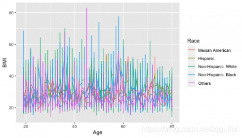
It is difficult to grasp anything in the plot above.

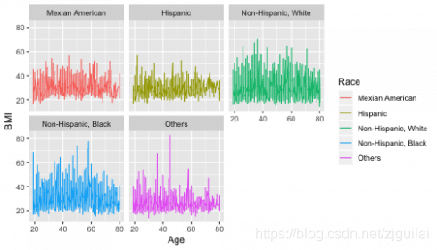
Let try to use the function facet_wrap to distinguish the race from each other.

facet_wrap

ggplot(dat, aes(x = Age, y = BMI)) + 
  geom_line(aes(color = Race)) +
  facet_wrap(~Race)

在这里插入图片描述
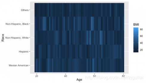
Heatmap
The geom_raster is the function to build a heatmap.

ggplot(dat, aes(Age, Race)) +
  geom_raster(aes(fill = BMI))

在这里插入图片描述
To give your own colors use the scale_fill_gradientn function.

ggplot(dat, aes(Age, Race)) +
  geom_raster(aes(fill = BMI)) +
  scale_fill_gradientn(colours=c("white", "red"))
  ![在这里插入图片描述](https://img-blog.csdnimg.cn/20190627162430900.png?x-oss-process=image/watermark,type_ZmFuZ3poZW5naGVpdGk,shadow_10,text_aHR0cHM6Ly9ibG9nLmNzZG4ubmV0L3pqZ3VpbGFp,size_16,color_FFFFFF,t_70)

传送门：https://datascienceplus.com/using-heatmap-to-simplify-the-data-visualization-in-r/