论文学习笔记（Densely Connected Convolutional Networks）

一.研究背景

解决梯度弥散（梯度消失问题）：

1.通过加深网络层数(VGG，ResNet)

2.加宽网络结构(GoogLeNet)来提升网络性能

创新点：

3.从特征的角度考虑, 通过特征重用和旁路(Bypass)设置

这样做的优点：

1.减轻了vanishing-gradient（梯度消失）

2、加强了feature的传递，更有效地利用了不同层的feature

3、网络更易于训练，并具有一定的正则效果.

4、因为整个网络并不深，所以一定程度上较少了参数数量

二.思想平台

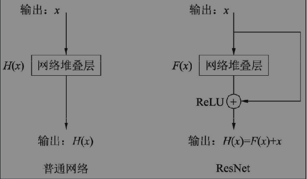
何恺明在提出ResNet时做出的假设: 若某一较深的网络多出另一较浅网络的若干层，且这些层有能力学习到恒等映射, 那么这一较深网络训练得到的模型性能一定不会弱于该浅层网络。DenseNet在提出时假设: 与其多次学习冗余的特征,特征复用是一种更好的特征提取方式。

Model Architecture

编辑切换为居中

添加图片注释，不超过 140 字（可选）

编辑切换为居中

添加图片注释，不超过 140 字（可选）

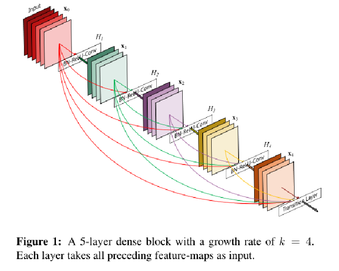
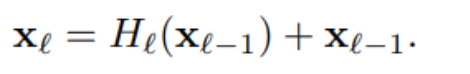
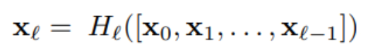
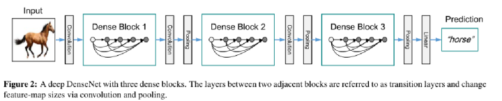
假设输入为一个图片X 0, 经过一个L层的神经网络, 第 l 层的特征输出记作 X l.

编辑

添加图片注释，不超过 140 字（可选）

编辑

添加图片注释，不超过 140 字（可选）

非线性变换H为BN+ReLU+ Conv(3×3)的组合。

Down-sampling Layer

编辑切换为居中

添加图片注释，不超过 140 字（可选）

DenseNet中需要对不同层的feature map进行cat操作,所以需要不同层的feature map保持相同的feature size,这就限制了网络中Down sampling的实现.为了使用Down sampling,作者将DenseNet分为多个stage，每个stage包含多个Dense blocks.

transition layers:由BN + Conv(kernel size 1×1) ＋ average-pooling(kernel size 2 x 2)组成.

1X1是为了对channel数量进行降维；而池化才是为了降低特征图的尺寸。

Growth rate

编辑切换为居中

添加图片注释，不超过 140 字（可选）

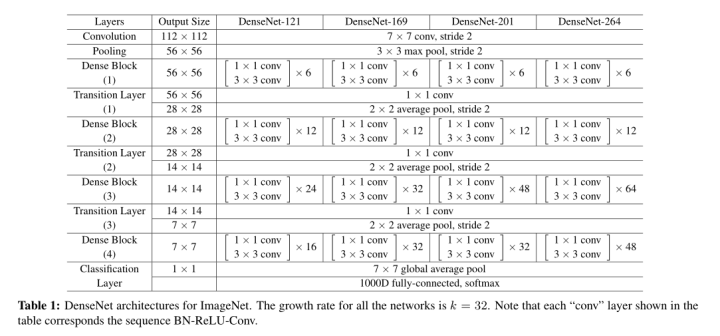
在Denseblock中,假设每一个卷积操作的输出为K个feature map, 那么第i层网络的输入便为(i-1)×K +（上一个Dense Block的输出channel）, 这个K在论文中的名字叫做Growth rate, 默认是等于32的

Note that each “conv” layer shown in the table corresponds the sequence BN-ReLU-Conv

Bottleneck layers:即BN-ReLU-Conv(1× 1)-BN-ReLU-Conv(3×3)

Model Comparation

编辑切换为居中

添加图片注释，不超过 140 字（可选）

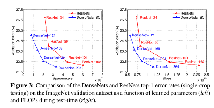
DenseNet与ResNet的对比图，在相同的错误率下，DenseNet的参数更少，计算复杂度也越低。

虽然DenseNet参数量少，但是训练过程中的中间产物（feature map）多

一.代码实现：

像Inception和ResNeXt一样，DenseNet使用BN-ReLU-Conv的结构代替传统的卷积层，本文所说的卷积层都表示的是BN-ReLU-Conv

# 定义基础卷积快
def conv_block(in_channel, out_channel):
    layer = nn.Sequential(
        nn.BatchNorm2d(in_channel),
        nn.ReLU(inplace=True),  # 提升训练速度，采用地址传递
        nn.Conv2d(in_channel, out_channel, kernel_size=3, padding=1, bias=False)
    )

Dense Block通过grow rate，卷积层数量L，输入特征层数三个参数控制：

class dense_block(nn.Module):
    def __init__(self, in_channel, growth_rate, num_layers):
        super(dense_block, self).__init__()
        block = []  # 放有多少个密集链接块
        channel = in_channel
        for i in range(num_layers):
            block.append(conv_block(channel, growth_rate))
            channel += growth_rate
        self.net = nn.Sequential(*block)

    def forward(self, X):
        for layer in self.net:
            out = layer(X)
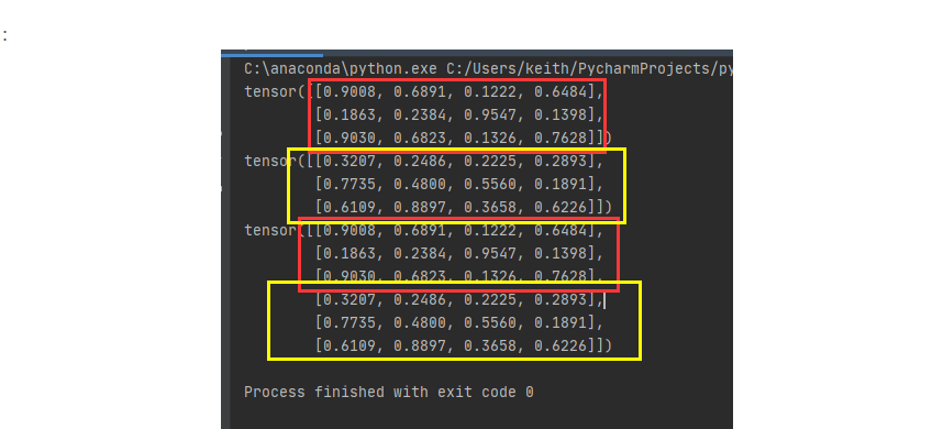
            X = torch.cat((out, X), dim=1)
        return X

.dim=0

编辑切换为居中

添加图片注释，不超过 140 字（可选）

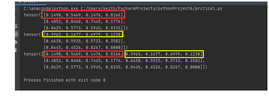
dim=1

编辑切换为居中

添加图片注释，不超过 140 字（可选）

编辑切换为居中

添加图片注释，不超过 140 字（可选）

transition层：由BN + Conv(kernel size 1×1) ＋ average-pooling(kernel size 2 x 2)组成.

def transition(in_channel, out_channel):
    trans_layer = nn.Sequential(
        nn.BatchNorm2d(),
        nn.ReLU(inplace=True),
        nn.Conv2d(in_channel, out_channel, 1),
        nn.AvgPool2d(2, 2)
    )
    return trans_layer

.图中有很多的dense_block块，transition_layer块，所以我们写成函数的， channels // 2就是为了降低复杂度。

def _make_transition_layer(self, channels):
    block = []
    block.append(transition(channels, channels // 2))

    return nn.Sequential(*block)

.densenet网络的全部流程

import torch
from torch import nn


# 定义基础卷积快
def conv_block(in_channel, out_channel):
    layer = nn.Sequential(
        nn.BatchNorm2d(in_channel),
        nn.ReLU(),  # 提升训练速度，采用地址传递
        nn.Conv2d(in_channel, out_channel, kernel_size=3, padding=1, bias=False)
    )
    return layer


class dense_block(nn.Module):
    def __init__(self, in_channel, growth_rate, num_layers):
        super(dense_block, self).__init__()
        block = []  # 放有多少个密集链接块
        channel = in_channel
        for i in range(num_layers):
            block.append(conv_block(channel, growth_rate))
            channel += growth_rate
        self.net = nn.Sequential(*block)

    def forward(self, X):
        for layer in self.net:
            out = layer(X)
            X = torch.cat((out, X), dim=1)
        return X


def transition(in_channel, out_channel):
    trans_layer = nn.Sequential(
        nn.BatchNorm2d(in_channel),
        nn.ReLU(),
        nn.Conv2d(in_channel, out_channel, 1),
        nn.AvgPool2d(2, 2)
    )
    return trans_layer


class densenet(nn.Module):
    def __init__(self, in_channel, num_classes, growth_rate=32, block_layer=[6, 12, 24, 16]):
        super(densenet, self).__init__()
        self.block1 = nn.Sequential(
            nn.Conv2d(in_channel, 64, 7, 2, 3),
            nn.BatchNorm2d(64),
            nn.ReLU(inplace=True),
            nn.MaxPool2d(3, 2, padding=1)
        )
        self.DB1 = self._make_dense_block(64, growth_rate, num=block_layer[0])
        self.TL1 = self._make_transition_layer(256)
        self.DB2 = self._make_dense_block(128, growth_rate, num=block_layer[1])
        self.TL2 = self._make_transition_layer(512)
        self.DB3 = self._make_dense_block(256, growth_rate, num=block_layer[2])
        self.TL3 = self._make_transition_layer(1024)
        self.DB4 = self._make_dense_block(512, growth_rate, num=block_layer[3])
        self.global_average = nn.Sequential(
            nn.BatchNorm2d(1024),
            nn.ReLU(),
            nn.AdaptiveAvgPool2d((1, 1))
        )
        self.classifier = nn.Linear(1024, num_classes)

    def forward(self, X):
        X = self.block1(X)
        X = self.DB1(X)
        X = self.TL1(X)
        X = self.DB2(X)
        X = self.TL2(X)
        X = self.DB3(X)
        X = self.TL3(X)
        X = self.DB4(X)
        X = self.global_average(X)
        X = X.view(X.shape[0], -1)  # 为了将前面多维度的tensor展平成一维
        X = self.classifier(X)

        return X

    def _make_dense_block(self, channels, growth_rate, num):
        block = []
        block.append(dense_block(channels, growth_rate, num))
        channels += num * growth_rate

        return nn.Sequential(*block)

    def _make_transition_layer(self, channels):
        block = []
        block.append(transition(channels, channels // 2))

        return nn.Sequential(*block)


# 测试代码
net = densenet(3, 10)
X = torch.rand(1, 3, 224, 224)
for name, layer in net.named_children():
    if name != "classifier":
        X = layer(X)
        print(name, 'output shape:', X.shape)
    else:
        X = X.view(X.size(0), -1)
        X = layer(X)
        print(name, 'output shape:', X.shape)

.数据集处理

import os
from shutil import copy
import random


def mkfile(file):
    if not os.path.exists(file):  # 判断路径是否存在
        os.makedirs(file)  # 创建指定目录名


file = "flower_photos/flower_photos"
flower_class = [cla for cla in os.listdir(file) if ".txt" not in cla]  # 复制文件名到列表中，但不包括txt格式
mkfile('flower_photos/train')
for cla in flower_class:
    mkfile('flower_photos/train/' + cla)
mkfile('flower_photos/val')
for cla in flower_class:
    mkfile('flower_photos/val/' + cla)

split_rate = 0.1
for cla in flower_class:  # 文件夹中 的第一层内容，也就是图片的种类
    cla_path = file + '/' + cla + '/'
    images = os.listdir(cla_path)  # 把图片放在相应的文件夹中
    num = len(images)
    evl_index = random.sample(images, k=int(num * split_rate))
    for index, image in enumerate(images):  # 提取图片
        if image in evl_index:
            image_path = cla_path + image
            new_path = 'flower_photos/val/' + cla
            copy(image_path, new_path)
        else:
            image_path = cla_path + image
            new_path = 'flower_photos/train/' + cla
            copy(image_path, new_path)
        print("[{}]processing [{}/{}]".format(cla, index + 1, num), end="")  # endl=""取消默认换行
    print()
print("processing done!")

.train代码

import time
import torch
import torch.nn as nn
import torchvision
import torchvision.transforms as transforms
import matplotlib.pyplot as plt
from model import Densenet
from torch.utils.data import DataLoader


def load_dataset(batch_size):
    train_set = torchvision.datasets.CIFAR10(
        root="data/cifar-10", train=True, download=True, transform=transforms.ToTensor()
    )
    test_set = torchvision.datasets.CIFAR10(
        root="data/cifar-10", train=False, download=True, transform=transforms.ToTensor()
    )
    train_iter = torch.utils.data.DataLoader(
        train_set, batch_size=batch_size, shuffle=True, num_workers=4
    )
    test_iter = torch.utils.data.DataLoader(
        test_set, batch_size=batch_size, shuffle=False, num_workers=4
    )
    return train_iter, test_iter


def train(net, train_iter, criterion, optimizer, num_epochs, device, num_print, lr_scheduler=None, test_iter=None):
    net.train()
    record_train = list()
    record_test = list()
    for epoch in range(num_epochs):
        print("============epoch:[{}/{}]===========".format(epoch + 1, num_epochs))
        total, correct, train_loss = 0, 0, 0
        start = time.time()
        for i, (X, y) in enumerate(train_iter):
            X, y = X.to(device), y.to(device)
            output = net(X)
            loss = criterion(output, y)

            optimizer.zero_grad()
            loss.backward()
            optimizer.step()

            train_loss += loss.item()
            total += y.size(0)
            correct += (output.argmax(dim=1) == y).sum().item()
            train_acc = 100.0 * correct / total
            if (i + 1) % num_print == 0:
                print("step: [{}/{}],train_loss : {:.3f} | train_acc : {:6.3f} %  | lr :{:.6f}"
                      .format(i + 1, len(train_iter), train_loss / (i + 1), train_acc, get_cur_lr(optimizer)))

        if lr_scheduler is not None:
            lr_scheduler.step()

        print("------cost time :{:.4f}s-----".format(time.time() - start))

        if test_iter is not None:
            record_test.append(test(net, test_iter, criterion, device))

    return record_train, record_test


def test(net, test_iter, criterion, device):
    total, correct = 0, 0
    net.eval()
    with torch.no_grad():
        print("**********test*******")
    for X, y in test_iter:
        X, y = X.to(device), y.to(device)

        output = net(X)
        loss = criterion(output, y)

        total += y.size(0)
        correct += (output.argmax(dim=1) == y).sum().item()

    test_acc = 100.0 * correct / total

    print("test_loss: {:.3f} | test_acc :{:6.3f}%".format(loss.item(), test_acc))
    print("******************")
    net.train()
    return test_acc


def get_cur_lr(optimizer):
    for param_group in optimizer.param_groups:
        return param_group["lr"]


def learning_curve(record_train, record_test=None):
    plt.style.use("ggplot")  # matplotlib.pyplot.style.use定制画布风格

    plt.plot(range(1, len(record_train) + 1), record_train, label="train acc")
    if record_test is not None:
        plt.plot(range(1, len(record_test) + 1), record_train, label="test acc")

    plt.legend(loc=4)
    plt.title("learning curve")
    plt.xticks(range(0, len(record_train) + 1, 5))
    plt.yticks(range(0, 101, 5))
    plt.xlabel("epoch")
    plt.ylabel("accuracy")

    plt.show()


import torch.optim as optim

BATCH_SIZE = 128
NUM_EPOCHS = 20
NUM_CLASSES = 10
LEARNING_RATE = 0.02
MOMENTUM = 0.9
WEIGHT_DECAY = 0.0005
NUM_PRINT = 100
DEVICE = "cuda" if torch.cuda.is_available() else "cpu"


def main():
    net = Densenet(NUM_CLASSES)
    net = net.to(DEVICE)

    train_iter, test_iter = load_dataset(BATCH_SIZE)

    criterion = nn.CrossEntropyLoss()
    optimizer = optim.SGD(net.parameters(), lr=LEARNING_RATE, momentum=MOMENTUM, weight_decay=WEIGHT_DECAY,
                          nesterov=True)
    lr_scheduler = optim.lr_scheduler.StepLR(optimizer, step_size=7, gamma=0.1)

    record_train, record_test = train(net, train_iter, criterion, optimizer, NUM_EPOCHS, DEVICE, NUM_PRINT,
                                      lr_scheduler, test_iter)
    learning_curve(record_train, record_test)


if __name__ == '__main__':
    main()