昇思25天学习打卡营第2天|张量Tensor

一、张量的定义：

张量是一种特殊的数据结构，与数组和矩阵非常相似。张量（Tensor）是MindSpore网络运算中的基本数据结构（也是所有深度学习模型的基础数据结构），下面将主要介绍张量和稀疏张量的属性及用法。 

张量（Tensor）是一个可用来表示在一些矢量、标量和其他张量之间的线性关系的多线性函数，这些线性关系的基本例子有内积、外积、线性映射以及笛卡儿积。其坐标在 𝑛 维空间内，有  N的R次方个分量的一种量，其中每个分量都是坐标的函数，而在坐标变换时，这些分量也依照某些规则作线性变换。R 称为该张量的秩或阶（与矩阵的秩和阶均无关系）。

二、环境准备：

import numpy as np
import mindspore
from mindspore import ops
from mindspore import Tensor, CSRTensor, COOTensor
import time

这里导入mindspore需要在本地先下载自己设备对应的MindSpore库，具体下载方法可以参考我的上一篇博客昇思25天学习打卡营第1天|快速入门。

三、创建张量：

张量的创建方式有多种，构造张量时，支持传入Tensor、float、int、bool、tuple、list和numpy.ndarray类型。下面我们使用mindspore提供的Tensor包，快速使用多种常见的tensor构建方式：

1、根据数据直接生成：

data = [1, 0, 1, 0]
x_data = Tensor(data)
print(x_data, x_data.shape, x_data.dtype)

# 官方打卡要求，可以自行修改
print(time.strftime('%Y-%m-%d %H:%M:%S', time.localtime(time.time())), "VertexGeek")

这段代码定义了一个名为data的列表，并通过mindspore的Tensor包直接转换成tensor张量形式，并打印这个张量，张量的维度，和张量的数据类型，效果如下： 

 2、由numpy数组生成：

这个方法和上面直接生成没什么区别，只是输入的数据由列表，变成了numpy数组。

np_array = np.array(data)
x_np = Tensor(np_array)
print(x_np, x_np.shape, x_np.dtype)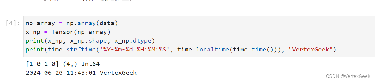

3、使用init初始化张量：

这个方法说直接一点就是通过mindspore的Tensor包直接构建张量，而不是先创造标量等数据之后再进行转换。

from mindspore.common.initializer import One, Normal

# 创建一个全是1的2×2的张量
tensor1 = mindspore.Tensor(shape=(2, 2), dtype=mindspore.float32, init=One())
# 创建一个服从正态分布的2×2的张量
tensor2 = mindspore.Tensor(shape=(2, 2), dtype=mindspore.float32, init=Normal())

print("tensor1:\n", tensor1)
print("tensor2:\n", tensor2)

print(time.strftime('%Y-%m-%d %H:%M:%S', time.localtime(time.time())), "VertexGeek")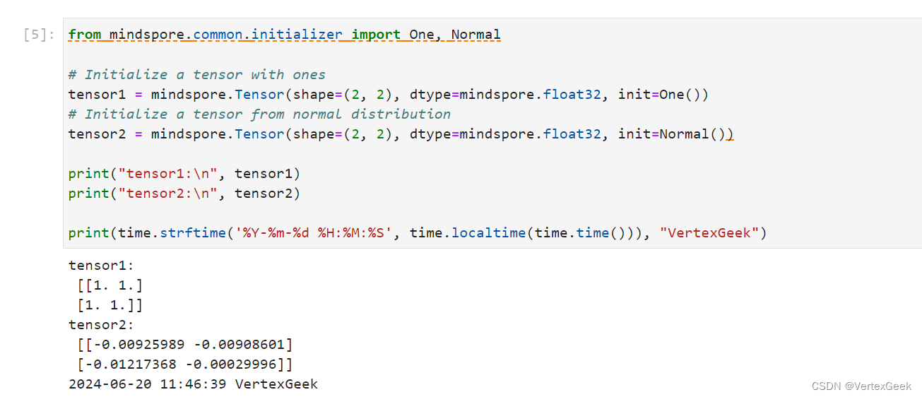

 

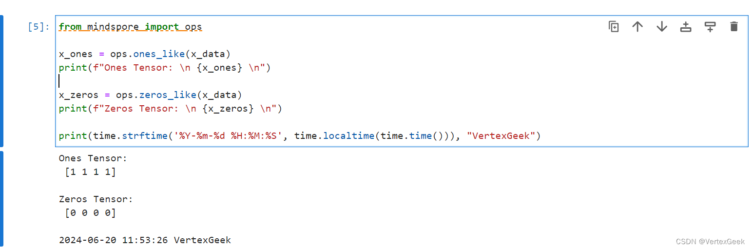
4、由张量构建张量：

这是一类最特殊的构建方式，但同时也非常常见，这次我们不是从非张量的数据如：列表、numpy数组等，构建张量，而是直接从张量到张量，有点绕，下面看代码（手动狗头） 

from mindspore import ops

x_ones = ops.ones_like(x_data)
print(f"Ones Tensor: \n {x_ones} \n")

x_zeros = ops.zeros_like(x_data)
print(f"Zeros Tensor: \n {x_zeros} \n")

print(time.strftime('%Y-%m-%d %H:%M:%S', time.localtime(time.time())), "VertexGeek")

 这里我们将由datal列表生成的x_data张量传入ops.ones_like（）方法中，构建一个全是1的维度和类型和x_data张量一样的张量，并命名为x_ones，ops.zeros_like的效果也是一样，生成的是全为0的张量。

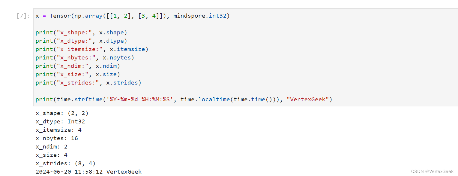
四、张量的属性：

张量的属性包括形状、数据类型、转置张量、单个元素大小、占用字节数量、维数、元素个数和每一维步长。

• 形状（shape）：Tensor的shape，是一个tuple。

• 数据类型（dtype）：Tensor的dtype，是MindSpore的一个数据类型。

• 单个元素大小（itemsize）： Tensor中每一个元素占用字节数，是一个整数。

• 占用字节数量（nbytes）： Tensor占用的总字节数，是一个整数。

• 维数（ndim）： Tensor的秩，也就是len(tensor.shape)，是一个整数。

• 元素个数（size）： Tensor中所有元素的个数，是一个整数。

• 每一维步长（strides）： Tensor每一维所需要的字节数，是一个tuple。

# 构建一个数据类型是int32，2×2的张量
x = Tensor(np.array([[1, 2], [3, 4]]), mindspore.int32)
# 打印张量的维度
print("x_shape:", x.shape)
# 打印张量的数据类型
print("x_dtype:", x.dtype)
# 打印单个元素大小
print("x_itemsize:", x.itemsize)
# 打印张量的字节数量
print("x_nbytes:", x.nbytes)
# 打印张量的维数
print("x_ndim:", x.ndim)
# 打印张量的元素总数
print("x_size:", x.size)
# 打印每一维度所需的字节数
print("x_strides:", x.strides)

print(time.strftime('%Y-%m-%d %H:%M:%S', time.localtime(time.time())), "VertexGeek")

打印结果： 

五、张量的索引：

 怎么说呢，和正常的数据索引基本一直。

tensor = Tensor(np.array([[0, 1], [2, 3]]).astype(np.float32))

print("First row: {}".format(tensor[0]))
print("value of bottom right corner: {}".format(tensor[1, 1]))
print("Last column: {}".format(tensor[:, -1]))
print("First column: {}".format(tensor[..., 0]))
print(time.strftime('%Y-%m-%d %H:%M:%S', time.localtime(time.time())), "VertexGeek")

tensor[0]：索引的是张量的第一个维度(计算机的索引从0开始)也就是[0,1] 

tensor[1,1]：索引的是张量的第二个维度的第二个数据也就是3

tensor[:, -1]：索引的是所有维度的第二个数据：1和3

tensor[..., 0]：索引的是所有维度的第一个数据：0和2

六、张量的计算：

张量之间有很多运算，包括算术、线性代数、矩阵处理（转置、标引、切片）、采样等，张量运算和NumPy的使用方式类似。

x = Tensor(np.array([1, 2, 3]), mindspore.float32)
y = Tensor(np.array([4, 5, 6]), mindspore.float32)

# 加（+）、减（-）、乘（*）、除（/）、取模（%）、整除（//）
output_add = x + y
output_sub = x - y
output_mul = x * y
output_div = y / x
output_mod = y % x
output_floordiv = y // x

print("add:", output_add)
print("sub:", output_sub)
print("mul:", output_mul)
print("div:", output_div)
print("mod:", output_mod)
print("floordiv:", output_floordiv)

print(time.strftime('%Y-%m-%d %H:%M:%S', time.localtime(time.time())), "VertexGeek")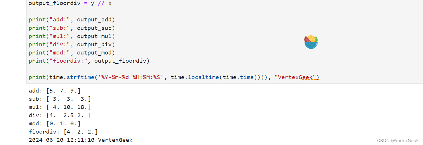

也可以通过concat和stack将两个张量连接起，concat将给定维度上的一系列张量连接起来 ,stack则是则是从另一个维度上将两个张量合并起来。

data1 = Tensor(np.array([[0, 1], [2, 3]]).astype(np.float32))
data2 = Tensor(np.array([[4, 5], [6, 7]]).astype(np.float32))
output1 = ops.concat((data1, data2), axis=0)
output2 = ops.stack([data1, data2])

print(output1)
print("shape:\n", output1.shape)
print(">>>>>>>>>>>>>>>>>")

print(output2)
print("shape:\n", output2.shape)
print(time.strftime('%Y-%m-%d %H:%M:%S', time.localtime(time.time())), "VertexGeek")

concat是根据两个张量的指定维度，将其拼接成一个张量，axis=0 就是按照第一个维度进行拼接

tensor和numpy之间可以互相转换：numpy转tensor之前已经展示了，下面是tensor转numpy的代码：

tensor = ops.Tensor(np.array([1., 1., 1., 1., 1.]).astype(np.float32))
numpy_array = tensor.asnumpy()

# 打印Tensor和NumPy数组的信息
print(f"t: {tensor} {type(tensor)}")
print(f"n: {numpy_array} {type(numpy_array)}")

print(time.strftime('%Y-%m-%d %H:%M:%S', time.localtime(time.time())), "VertexGeek")

 七、稀疏张量：

稀疏张量是一种特殊张量，其中绝大部分元素的值为零。

在某些应用场景中（比如推荐系统、分子动力学、图神经网络等），数据的特征是稀疏的，若使用普通张量表征这些数据会引入大量不必要的计算、存储和通讯开销。这时就可以使用稀疏张量来表征这些数据。

MindSpore现在已经支持最常用的CSR和COO两种稀疏数据格式。

常用稀疏张量的表达形式是<indices:Tensor, values:Tensor, shape:Tensor>。其中，indices表示非零下标元素， values表示非零元素的值，shape表示的是被压缩的稀疏张量的形状。在这个结构下，我们定义了三种稀疏张量结构：CSRTensor、COOTensor和RowTensor。

1、CSRTensor:

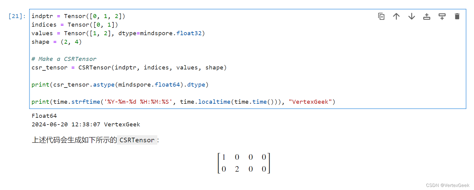
CSR（Compressed Sparse Row）稀疏张量格式有着高效的存储与计算的优势。其中，非零元素的值存储在values中，非零元素的位置存储在indptr（行）和indices（列）中。

indptr = Tensor([0, 1, 2])
indices = Tensor([0, 1])
values = Tensor([1, 2], dtype=mindspore.float32)
shape = (2, 4)

# 创建一个CSRTensor的稀疏张量
csr_tensor = CSRTensor(indptr, indices, values, shape)

print(csr_tensor.astype(mindspore.float64).dtype)

print(time.strftime('%Y-%m-%d %H:%M:%S', time.localtime(time.time())), "VertexGeek")

indptr = Tensor([0, 1, 2])：第一行的非零元素是values中第一个元素，第二行的非零元素是value中的第二个元素，第三行及以后的行对应value中的第三个元素（这里我们的value只有两个，所以不会继续构建张量）。

indices = Tensor([0, 1])：规定了第一个非零元素位于第一列，第二个非零元素位于第二列，注意indices输入的参数数量必须和values输入的参数量一致。

2、COOTensor:

COO（Coordinate Format）稀疏张量格式用来表示某一张量在给定索引上非零元素的集合，若非零元素的个数为N，被压缩的张量的维数为ndims。

indices = Tensor([[0, 1], [1, 2]], dtype=mindspore.int32)
values = Tensor([1, 2], dtype=mindspore.float32)
shape = (3, 4)

# Make a COOTensor
coo_tensor = COOTensor(indices, values, shape)

print(coo_tensor.values)
print(coo_tensor.indices)
print(coo_tensor.shape)
print(coo_tensor.astype(mindspore.float64).dtype)  # COOTensor to float64

print(time.strftime('%Y-%m-%d %H:%M:%S', time.localtime(time.time())), "VertexGeek")

张量是深度学习的基础，学习好tensor有利于后面的学习。