运用lstm预测黄金和比特币价格

       由于对数学建模比较感兴趣，并且有参加一些数学建模的比赛，于是在闲着无聊的时候我会去找一些算法和模型的代码进行修改并且尝试跑一跑，对一些特定问题进行求解。在2022年的美赛c题里，给到了黄金和比特币的一些数据，并且观察过问题之后发现其中需要预测模型，由于以前没接触过lstm模型，于是便尝试运用lstm对黄金和比特币的价格进行预测。

       这里简单介绍一下lstm模型，知乎、本网站其实已经有很多人有非常详细的介绍，于是我在这里就简明地介绍一下：

lstm，中文名字叫做长短期记忆模型，是一种特殊的RNN模型，通过引入门机制，解决了RNN模型不具备的长记忆性问题，大致结构如图（此图转载至知乎的一篇文章，如果制作者不想我用的话可以私信我删除）：

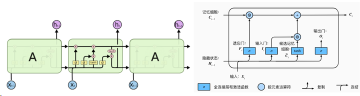
lstm 拥有三个门，来保护和控制细胞状态：遗忘门、更新门和输出门，门机制是让信息选择式通过的方法，通过sigmoid函数和点乘操作实现。sigmoid取值介于0～1之间，乘即点乘则决定了传送的信息量（每个部分有多少量可以通过），当sigmoid取0时表示舍弃信息，取1时表示完全传输(即完全记住)。具体三个门怎么运转的，大家可以参考其他的博客，很多人都写的非常详细的。

       接下来就介绍本篇文章的重点，运用lstm来预测16-21年的黄金和比特币的数据，由于赛题里说只能用赛题提供的数据，所以这里我们训练数据和用来预测的数据均用同一个，但大家在平时使用的时候要自己收集以往的数据或者通过现有数据进行划分来作为训练集，这里提供一个黄金和比特币收集数据的平台，里面的数据非常全面：英为财情Investing.com_全球金融行情资讯专家|外汇,股票,期货,债券,数字货币行情和财经新闻

这里我就不提供我这里用的数据了，如果要使用的话可以直接去美赛的官网找2022年的赛题数据，或者直接用上面网址的数据。这里用的代码是从网上寻找适合的然后进行相应的修改的，大家有更好的代码也可以在评论区里留言。

为了能让使用者在较早的时间更快获取预测数据，我把观察的跨度设置为2，即根据前2天的数据对下一天的数据进行预测，我这里先对数据进行标准化，并求解模型的损失函数来查看模型的精确度和拟合度，我采用均方误差损失进行损失函数的求解与绘制，以下为代码部分：

import numpy as np
import pandas as pd
import matplotlib.pyplot as plt


filepath = 'E:\desktop\chain1.csv'
data = pd.read_csv(filepath)
data = data.sort_values('Date')
print(data.head())
print(data.shape)


price = data[['Value']]
print(price.info())

from sklearn.preprocessing import MinMaxScaler

# 进行不同的数据缩放，将数据缩放到-1和1之间
scaler = MinMaxScaler(feature_range=(-1, 1))
price['Value'] = scaler.fit_transform(price['Value'].values.reshape(-1, 1))
print(price['Value'].shape)


# 数据集制作
# lookback表示观察的跨度
def split_data(stock, lookback):
    data_raw = stock.to_numpy()
    data = []
    # print(data)

    # you can free play（seq_length）
    for index in range(len(data_raw) - lookback):
        data.append(data_raw[index: index + lookback])

    data = np.array(data);
    test_set_size = data.shape[0]
    train_set_size = data.shape[0]

    x_train = data[:train_set_size, :-1, :]
    y_train = data[:train_set_size, -1, :]

    x_test = data[:train_set_size, :-1, :]
    y_test = data[:train_set_size, -1, :]

    return [x_train, y_train, x_test, y_test]


lookback = 2
x_train, y_train, x_test, y_test = split_data(price, lookback)
print('x_train.shape = ', x_train.shape)
print('y_train.shape = ', y_train.shape)
print('x_test.shape = ', x_test.shape)
print('y_test.shape = ', y_test.shape)

# 模型构建 —— LSTM

import torch
import torch.nn as nn

x_train = torch.from_numpy(x_train).type(torch.Tensor)
x_test = torch.from_numpy(x_test).type(torch.Tensor)
y_train_lstm = torch.from_numpy(y_train).type(torch.Tensor)
y_test_lstm = torch.from_numpy(y_test).type(torch.Tensor)
y_train_gru = torch.from_numpy(y_train).type(torch.Tensor)
y_test_gru = torch.from_numpy(y_test).type(torch.Tensor)
# 输入的维度为1，只有Value
input_dim = 1
# 隐藏层特征的维度
hidden_dim = 32
# 循环的layers
num_layers = 2
# 预测后一天的Value
output_dim = 1
num_epochs = 100


class LSTM(nn.Module):
    def __init__(self, input_dim, hidden_dim, num_layers, output_dim):
        super(LSTM, self).__init__()
        self.hidden_dim = hidden_dim
        self.num_layers = num_layers

        self.lstm = nn.LSTM(input_dim, hidden_dim, num_layers, batch_first=True)
        self.fc = nn.Linear(hidden_dim, output_dim)

    def forward(self, x):
        h0 = torch.zeros(self.num_layers, x.size(0), self.hidden_dim).requires_grad_()
        c0 = torch.zeros(self.num_layers, x.size(0), self.hidden_dim).requires_grad_()
        out, (hn, cn) = self.lstm(x, (h0.detach(), c0.detach()))
        out = self.fc(out[:, -1, :])
        return out


model = LSTM(input_dim=input_dim, hidden_dim=hidden_dim, output_dim=output_dim, num_layers=num_layers)
criterion = torch.nn.MSELoss()
optimiser = torch.optim.Adam(model.parameters(), lr=0.01)

# 模型训练
import time

hist = np.zeros(num_epochs)
start_time = time.time()
lstm = []

for t in range(num_epochs):
    y_train_pred = model(x_train)

    loss = criterion(y_train_pred, y_train_lstm)
    print("Epoch ", t, "MSE: ", loss.item())
    hist[t] = loss.item()

    optimiser.zero_grad()
    loss.backward()
    optimiser.step()

training_time = time.time() - start_time
print("Training time: {}".format(training_time))

# 模型结果可视化

predict = pd.DataFrame(scaler.inverse_transform(y_train_pred.detach().numpy()))
original = pd.DataFrame(scaler.inverse_transform(y_train_lstm.detach().numpy()))

import seaborn as sns

sns.set_style("darkgrid")

fig = plt.figure()
fig.subplots_adjust(hspace=0.2, wspace=0.2)

plt.subplot(1, 2, 1)
ax = sns.lineplot(x=original.index, y=original[0], label="Data", color='royalblue')
ax = sns.lineplot(x=predict.index, y=predict[0], label="Training Prediction (LSTM)", color='tomato')
# print(predict.index)
# print(predict[0])


ax.set_title('Stock price', size=14, fontweight='bold')
ax.set_xlabel("Days", size=14)
ax.set_ylabel("Cost (USD)", size=14)
ax.set_xticklabels('', size=10)

plt.subplot(1, 2, 2)
ax = sns.lineplot(data=hist, color='royalblue')
ax.set_xlabel("Epoch", size=14)
ax.set_ylabel("Loss", size=14)
ax.set_title("Training Loss", size=14, fontweight='bold')
fig.set_figheight(6)
fig.set_figwidth(16)
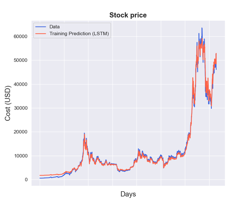
plt.show()

比特币数据的原数据与预测数据图：

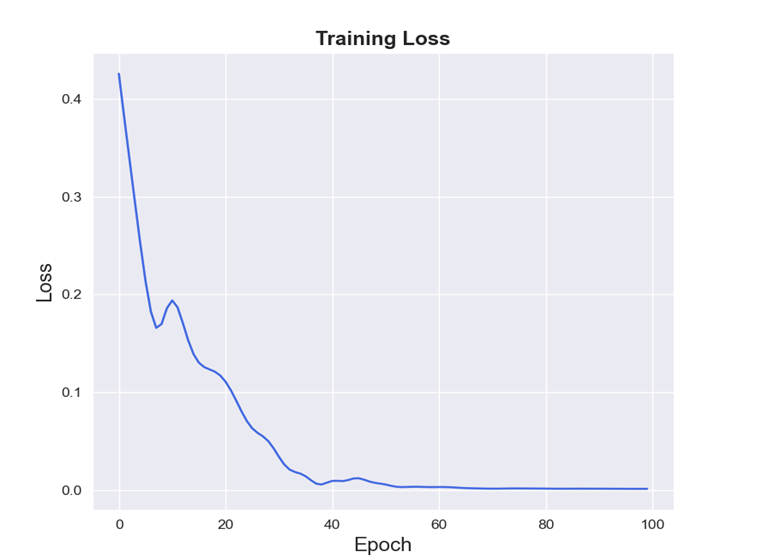
比特币数据的损失函数图：

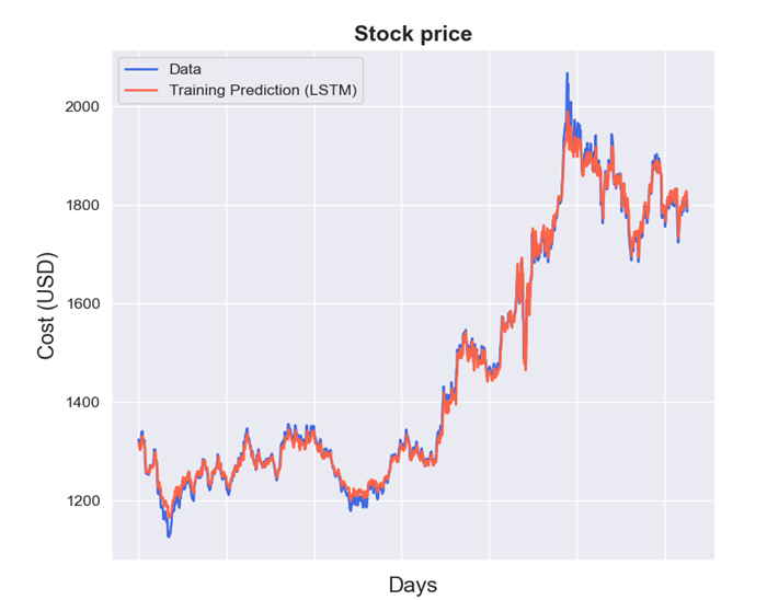
黄金数据的原数据与预测数据图：

黄金数据的损失函数图：

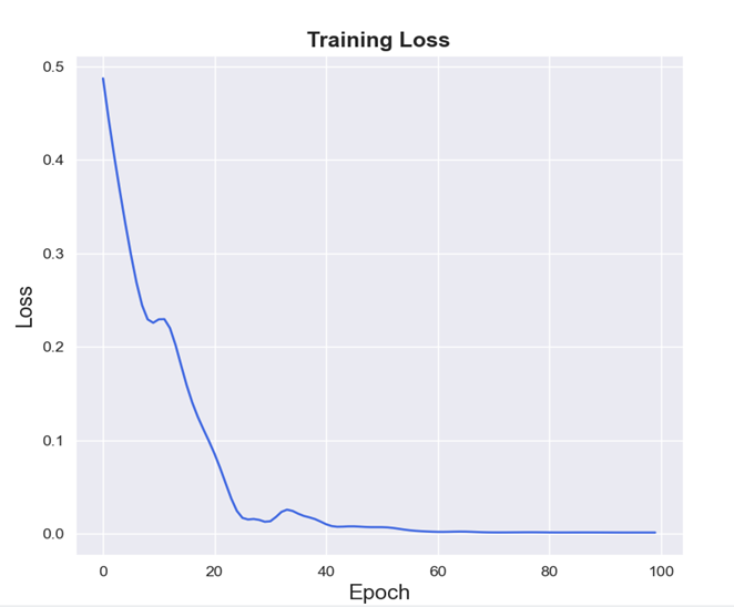
       由图可看出，比特币与黄金的预测值拟合效果良好，损失函数值均低于0.5，较小，模型精确度良好。

这里提供一些比较显而易见的可以根据实际情况改变的地方： 

1.lookback值，看你是需要运用前x个预测后一个的值，lookback=x       

2.Date和Value为原数据里的Date列和Value（比特币或黄金的价格）列，需根据实际情况修改

3.训练集和测试集分别要弄多少个，在这个地方进行修改：

data = np.array(data);
test_set_size = data.shape[0]
train_set_size = data.shape[0]

       当然，我这里展示的lstm模型是没有更细致的加入优化算法的，如果想研究更深入的话可以尝试添加一些智能优化算法改进，比如经典的三件套：模拟退火、遗传、粒子群，后续我也可能会进行相应的研究。并且模型具有滞后性，需要根据实际情况调整模型参数来解决此问题，由于金融市场的波动与不稳定性，模型预测结果并不能非常准确地反映金融市场的变动。