基于机器学习的Bitcoin价格预测（Python）

基于机器学习的Bitcoin价格预测（Python）

Import Libraries and Data

import numpy as np
import matplotlib.pyplot as plt
import pandas as pd
import seaborn as sns
import warnings
warnings.filterwarnings('ignore')
data=pd.read_csv('bitcoin_price_bitcoin_price.2013Apr-2017Aug.csv',index_col='Date')
data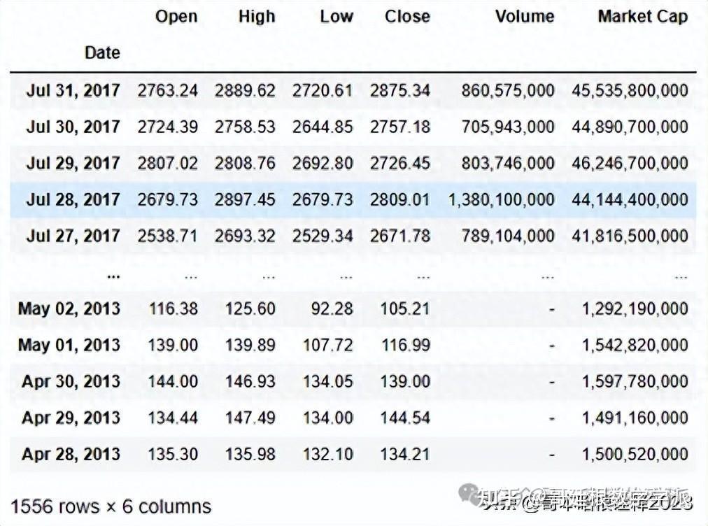

Data Analysis

accuracy_arr=[]#array to store accuracy
data.info()
<class 'pandas.core.frame.DataFrame'>
Index: 1556 entries, Jul 31, 2017 to Apr 28, 2013
Data columns (total 6 columns):
 #   Column      Non-Null Count  Dtype  
---  ------      --------------  -----  
 0   Open        1556 non-null   float64
 1   High        1556 non-null   float64
 2   Low         1556 non-null   float64
 3   Close       1556 non-null   float64
 4   Volume      1556 non-null   object 
 5   Market Cap  1556 non-null   object 
dtypes: float64(4), object(2)
memory usage: 85.1+ KB
data.describe()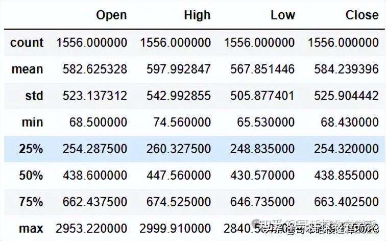

Preprocessing

data=data.drop(['Volume','Market Cap'],axis=1)
data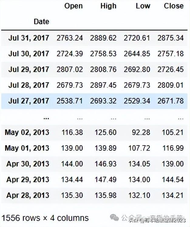

data.index=pd.to_datetime(data.index)
data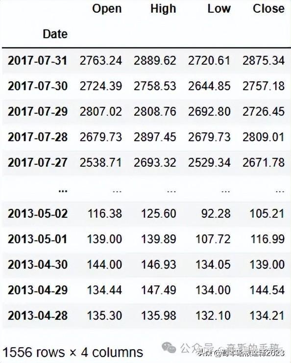

data = data.sort_index()
data.head()

	Open	High	Low	Close
Date
2013-04-28	135.30	135.98	132.10	134.21
2013-04-29	134.44	147.49	134.00	144.54
2013-04-30	144.00	146.93	134.05	139.00
2013-05-01	139.00	139.89	107.72	116.99
2013-05-02	116.38	125.60	92.28	105.21

Plot of Bitcoin price vs Date

plt.figure(figsize=(12,6))
data['Close'].plot()


plt.ylabel("Daily Bitcoin price")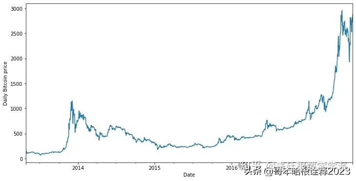

data=data.drop(['Open','High','Low',],axis=1) ##drop the open, high and low
data

	Close
Date
2013-04-28	134.21
2013-04-29	144.54
2013-04-30	139.00
2013-05-01	116.99
2013-05-02	105.21
...	...
2017-07-27	2671.78
2017-07-28	2809.01
2017-07-29	2726.45
2017-07-30	2757.18
2017-07-31	2875.34

1556 rows × 1 columns

Generating Features

columns_name=['f1','f2','f3','f4','f5']
new=data
for i in range(1,6):
  data[columns_name[i-1]]=data['Close'].shift(periods=-i)
data.tail(10)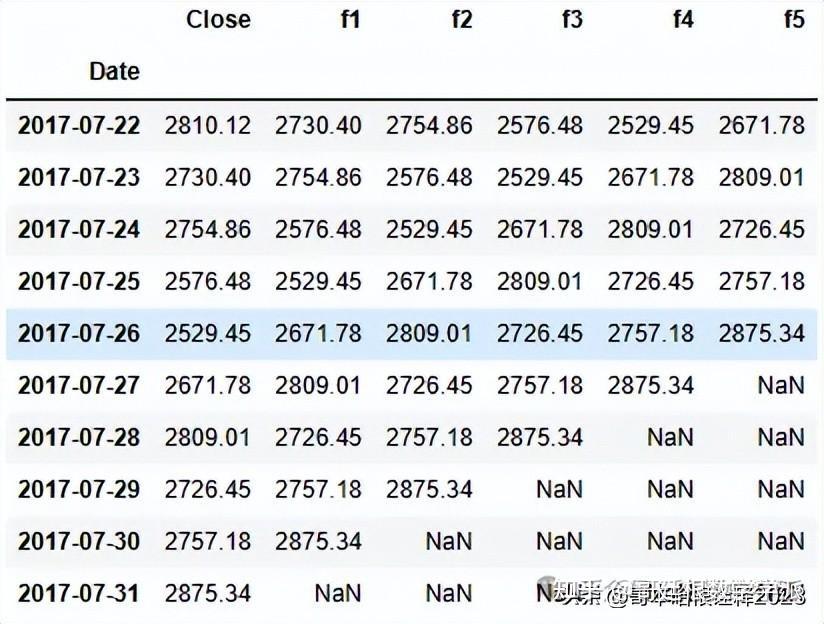

data=data.iloc[0:len(data)-5,:]

Scaling

from sklearn.preprocessing import MinMaxScaler
scaler = MinMaxScaler()
scaler.fit(data)
data=scaler.transform(data)
data=pd.DataFrame(data,columns=[['Close','f1','f2','f3','f4','f5']])
x=data.iloc[:,[1,2,3,4,5]]
y=data.iloc[:,[0]]
x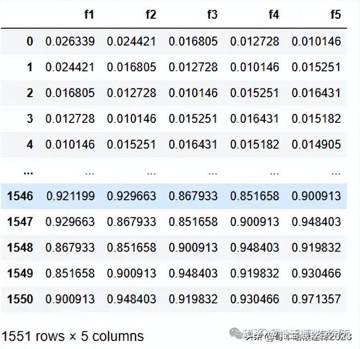

Train Test Split

train_size = int(len(data) * 0.7)
test_size = len(data) - train_size
train, test = data.iloc[0:train_size,:], data.iloc[train_size:len(data),:]
x_train=train.iloc[:,[1,2,3,4,5]]
y_train=train.iloc[:,[0]]
x_test=test.iloc[:,[1,2,3,4,5]]
y_test=test.iloc[:,[0]]

Decision Tree Classifier

Decision Tree Classifier with different hyperparameters

from sklearn.tree import DecisionTreeRegressor
from sklearn import metrics
Criterion=['squared_error']


for info in Criterion:
  for i in range (5,15):
    for j in range (2,10):
      for k in range (2,20):
        cls=DecisionTreeRegressor(criterion=info, max_depth=i,max_leaf_nodes=2*k,min_samples_split=j,random_state=42)
        cls.fit(x_train,y_train)
        y_pred=cls.predict(x_test)
        x_pred=cls.predict(x_train)
        # if metrics.r2_score(y_test,y_pred)>0.3:
        print(info,i,j,k,metrics.r2_score(y_test,y_pred))
squared_error 14 9 9 0.27741862551731833
squared_error 14 9 10 0.27749566394131886
squared_error 14 9 11 0.277387184544298
squared_error 14 9 12 0.2776277578525831
squared_error 14 9 13 0.27762221885488847
squared_error 14 9 14 0.27644323078170563
squared_error 14 9 15 0.2764806120616359
squared_error 14 9 16 0.27654989524362195
squared_error 14 9 17 0.27654989524362195
squared_error 14 9 18 0.27654989524362195
squared_error 14 9 19 0.27663449679360885
from sklearn.tree import DecisionTreeRegressor
dtree = DecisionTreeRegressor(criterion='squared_error', max_depth=8,max_leaf_nodes=16,min_samples_split=2,random_state=42)
dtree.fit(x_train,y_train)
y_pred=dtree.predict(x_test)
metrics.r2_score(y_test,y_pred)
0.279281936679907
accuracy_arr.append(metrics.r2_score(y_test,y_pred))
y_pred=pd.DataFrame(y_pred)
# plt.figure(figsize=(12,6))
y_test=np.array(y_test)
y_pred=np.array(y_pred)

Plot to compare price vs Days

plt.figure(figsize=(12,6))
plt.plot(np.array(range(466)),y_test,label='Original')
plt.plot(np.array(range(466)),y_pred,label='Predicted')
plt.legend()
plt.xlabel('Days')
plt.ylabel('Price(Scaled)')
plt.show()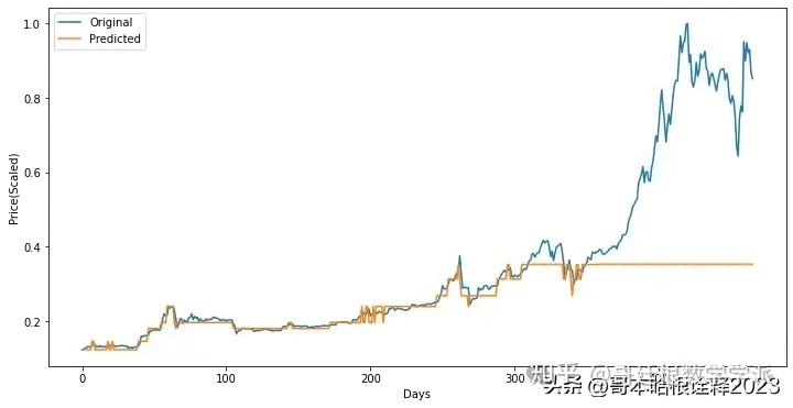

XGB (Shallow)

Implement model with differnet learning rate

import xgboost as xgb
for i in range(1,40):
  XGB = xgb.XGBRegressor(max_depth=2,learning_rate=0.01*i)
  XGB.fit(x_train,y_train)
  y_pred=XGB.predict(x_test)
  k=XGB.predict(x_train)
  print(metrics.r2_score(y_test,y_pred),i)
XGB = xgb.XGBRegressor(max_depth=2,learning_rate=0.01*35)
XGB.fit(x_train,y_train)
y_pred=XGB.predict(x_test)
k=XGB.predict(x_train)
print(metrics.r2_score(y_test,y_pred))
accuracy_arr.append(metrics.r2_score(y_test,y_pred))

Plot of Price vs Days

plt.figure(figsize=(12,6))
plt.plot(np.array(range(466)),y_test,label='Original')
plt.plot(np.array(range(466)),y_pred,label='Predicted')
plt.xlabel('Days')
plt.ylabel('Price(Scaled)')
plt.legend()
plt.show()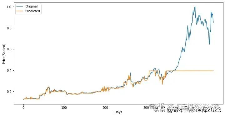

XGB (Deep)

import xgboost as xgb
for i in range(1,40):
  XGB = xgb.XGBRegressor(max_depth=12,learning_rate=0.01*i)
  XGB.fit(x_train,y_train)
  y_pred=XGB.predict(x_test)
  k=XGB.predict(x_train)
  print(metrics.r2_score(y_test,y_pred),i)
[15:46:51] WARNING: /workspace/src/objective/regression_obj.cu:152: reg:linear is now deprecated in favor of reg:squarederror.
0.33455680167499247 35
[15:46:51] WARNING: /workspace/src/objective/regression_obj.cu:152: reg:linear is now deprecated in favor of reg:squarederror.
0.33621573823007167 36
[15:46:52] WARNING: /workspace/src/objective/regression_obj.cu:152: reg:linear is now deprecated in favor of reg:squarederror.
0.307782864222201 37
[15:46:52] WARNING: /workspace/src/objective/regression_obj.cu:152: reg:linear is now deprecated in favor of reg:squarederror.
0.30853605662649164 38
[15:46:52] WARNING: /workspace/src/objective/regression_obj.cu:152: reg:linear is now deprecated in favor of reg:squarederror.
0.3007506935530976 39
XGB = xgb.XGBRegressor(max_depth=12,learning_rate=0.01*26)
XGB.fit(x_train,y_train)
y_pred=XGB.predict(x_test)
k=XGB.predict(x_train)
print(metrics.r2_score(y_test,y_pred))

Plot of Price vs Days

plt.figure(figsize=(12,6))
plt.plot(np.array(range(466)),y_test,label='Original')
plt.plot(np.array(range(466)),y_pred,label='Predicted')
plt.xlabel('Days')
plt.ylabel('Price(Scaled)')
plt.legend()
plt.show()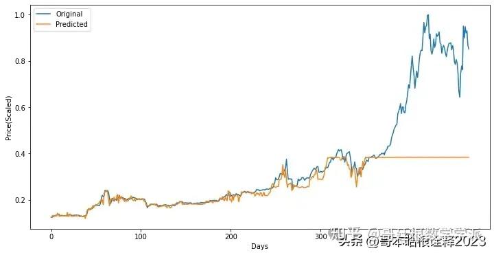

Linear Regression

Implement Model

from sklearn.linear_model import LinearRegression
reg=LinearRegression()
reg.fit(x_train,y_train)
y_pred=reg.predict(x_test)
print(metrics.r2_score(y_test,y_pred))
0.9926650271996021
accuracy_arr.append(metrics.r2_score(y_test,y_pred))

Plot of Price vs Days

plt.figure(figsize=(12,6))
plt.plot(np.array(range(466)),y_test,label='Original')
plt.plot(np.array(range(466)),y_pred,label='Predicted')
plt.xlabel('Days')
plt.ylabel('Price(Scaled)')
plt.legend()
plt.show()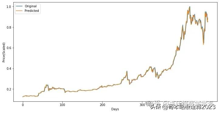

Random Forest

Implement Random Forest with hyperparameters

from sklearn.ensemble import RandomForestRegressor


clf = RandomForestRegressor(max_depth=6, random_state=0,n_estimators=500)
clf.fit(x_train,y_train)
y_pred=clf.predict(x_test)
metrics.r2_score(y_test,y_pred)
0.22059311748223798
accuracy_arr.append(metrics.r2_score(y_test,y_pred))

Plot of Price vs Days

plt.figure(figsize=(12,6))
plt.plot(np.array(range(466)),y_test,label='Original')
plt.plot(np.array(range(466)),y_pred,label='Predicted')
plt.xlabel('Days')
plt.ylabel('Price(Scaled)')
plt.legend()
plt.show()

LSTM

Import Libraries

from keras.models import Sequential
from keras.layers import Dense
from keras.layers import LSTM
x_train=np.array(x_train)
x_test=np.array(x_test)

Change shape of numpy array

trainX = np.reshape(x_train, (x_train.shape[0], 1, x_train.shape[1]))
testX = np.reshape(x_test, (x_test.shape[0], 1, x_test.shape[1]))
testY=np.array(y_test)
trainY=np.array(y_train)

Implement LSTM model

lstm = Sequential()
lstm.add(LSTM(100, input_shape=(trainX.shape[1], trainX.shape[2])))
lstm.add(Dense(1))
lstm.compile(loss='mae', optimizer='adam')
lstm.fit(trainX, trainY, epochs=300, batch_size=100, verbose=0, shuffle=False)

Plot of Price vs Days for comparision

y_pred = lstm.predict(testX)
plt.figure(figsize=(12,6))
plt.plot(y_pred, label='predicted')
plt.plot(testY, label='original')
plt.xlabel('Days')
plt.ylabel('Price(Scaled)')
plt.legend()
plt.show()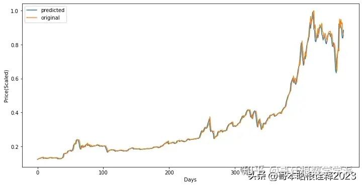

R2 score Plot

models=['DTR','XGB(Shallow)','XGB(Deep)','Linear Regressor','Random Forest','LSTM']
fig = plt.figure(figsize = (10, 5))
plt.bar(models,accuracy_arr ,width = 0.4)
 
plt.xlabel("Models")
plt.ylabel("R2 Score")


plt.show()

学术咨询：

担任《Mechanical System and Signal Processing》《中国电机工程学报》等期刊审稿专家，擅长领域：信号滤波/降噪，机器学习/深度学习，时间序列预分析/预测，设备故障诊断/缺陷检测/异常检测。

分割线分割线分割线分割线分割线分割线

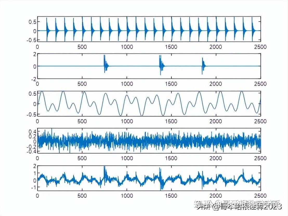
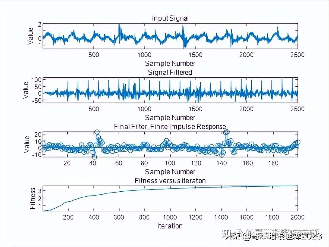
一种基于优化盲反褶积的旋转机械振动信号滤波降噪方法（MATLAB）

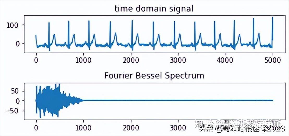
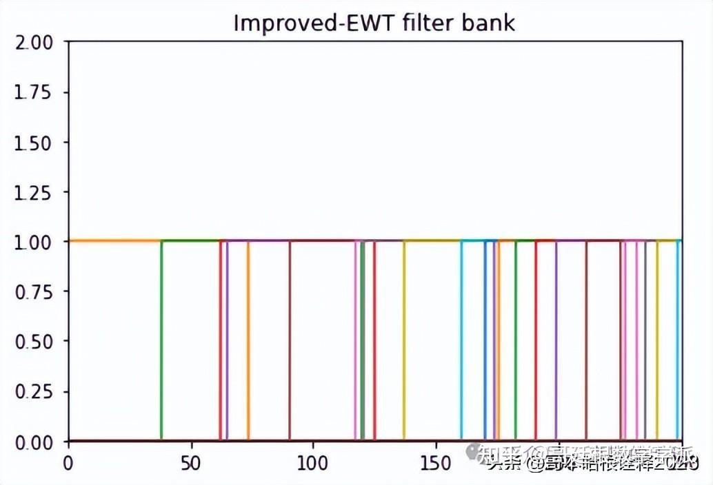
一种基于傅里叶贝塞尔级数展开的经验小波变换方法（Python）

完整代码可通过学术咨询获得：