黎曼猜想为什么重要

黎曼猜想联系上千个数学命题

迄今为止，有上千个数学命题以黎曼猜想及其推广形式的成立为前提，如果黎曼猜想被证实，那么数学家们长期建立在此猜想上而计算出的一切公式、结论都将被证实，并将会把它们运用到金融、人工智能、生物神经网络、国家保密系统等多个十分重要并且尖端的先进高科技领域，从而推动整个社会的发展．与此相反，如果黎曼猜想被推翻，那么这些数学命题中绝大多数将会不可避免地成为“陪葬”品．并且，黎曼猜想的证实，可能促使更多数学规律的发现，开辟更多数学领域，解决更多数学难题，得出更多结论。

黎曼猜想直接影响数论的发展

数论是传统数学的一个重要分支，曾被高斯称作“数学中的女皇”，而质数分布问题是数论的一个重点研究课题．对质数的研究可以追溯到古希腊时期，欧几里得用反证法证明了自然数中存在着无穷多个质数，但是对质数的分布规律却毫无头绪．后续众多数学家对特立独行的质数极为感兴趣，期待研究清楚质数的分布，这就使得黎曼猜想在科学家们心目中的地位和重要性大大提升。

曼猜想“侵入”到物理学领地

早在20世纪70年代，有科学家发现黎曼猜想与某些物理现象存在关联，基于黎曼猜想产生了一些十分惊艳的想法，很多物理学中的重要命题可以在黎曼猜想成立的前提下得到证明．如所有自然数的和，即1+2+3+⋯通过黎曼r函数的解析延拓可产生看似荒谬的结果-1/12。这一结论在量子力学和弦论等领域已有所应用．可以说黎曼猜想的证明是无数数学家和物理学家都关注的议题。

学术咨询：

担任《Mechanical System and Signal Processing》《中国电机工程学报》等期刊审稿专家，擅长领域：信号滤波/降噪，机器学习/深度学习，时间序列预分析/预测，设备故障诊断/缺陷检测/异常检测。

海面水温序列的连续小波变换（Python，ipynb文件）

海面水温序列的连续小波变换（Python，ipynb文件）

import numpy as np
from waveletFunctions import wavelet, wave_signif
import matplotlib.pyplot as plt
​
sst = np.loadtxt('sst_nino3.dat')
n = len(sst)
dt = 0.25
time = np.arange(len(sst)) * dt + 1871.0  # array of time epochs
xlim = ([1870, 2000])
​
​
%matplotlib inline
plt.figure(figsize=(12, 4))
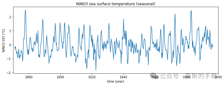
plt.plot(time, sst)
plt.xlim(xlim[:])
plt.xlabel('time (year)')
plt.ylabel('NINO3 SST (°C)')
plt.title('NINO3 sea surface temperature (seasonal)')
plt.show()

Scaling

pad = 1  # zero padding (recommended)
dj = 0.125  # 8 sub-octaves (within one octave)
s0 = 2 * dt  # 6 month initial scale
j1 = 7 / dj  # 7 octaves
mother = 'MORLET'

Continuous wavelet transform

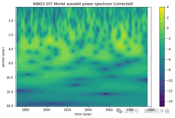
# Wavelet transform:
wave, period, scale, coi = wavelet(sst, dt, pad, dj, s0, j1, mother)
power = (np.abs(wave)) ** 2  # power spectrum (not quite correct)
scale_ext = np.outer(scale,np.ones(n))
power = (np.abs(wave))**2 /scale_ext  # power spectrum (corrected)

Plot wavelet power spectrum

#--- wavelet power spectrum (contour and color plot)
import matplotlib
plt.figure(figsize=(10, 6))
levels = np.array([2**i for i in range(-15,5)])
CS
 = plt.contourf(time, period, np.log2(power), len(levels))  
#*** or 'contour'
im = plt.contourf(CS, levels=np.log2(levels))
# im = plt.imshow(np.log2(np.flipud(power)),extent=[1870, 2000, 0.5, 64])
plt.xlabel('time (year)')
plt.ylabel('period (year)')
plt.title('NINO3 SST Morlet wavelet power spectrum (corrected)')
plt.xlim(xlim[:])
plt.yscale('log', base=2, subs=None)
plt.ylim([np.min(period), np.max(period)])
ax = plt.gca().yaxis
ax.set_major_formatter(matplotlib.ticker.ScalarFormatter())
plt.ticklabel_format(axis='y', style='plain')
plt.gca().invert_yaxis()
plt.colorbar(im, orientation='vertical')
plt.show()

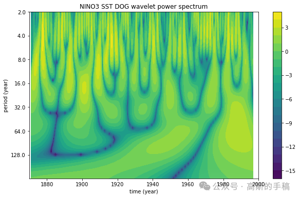
mother = 'DOG'
wave1, period1, scale1, coi1 = wavelet(sst, dt, pad, dj, s0, j1, mother)
power1 = (np.abs(wave1)) ** 2
​
# plot
plt.figure(figsize=(10, 6))
levels = np.array([2**i for i in range(-16,6)])
CS = plt.contourf(time, period1, np.log2(power1), len(levels))  #*** or 'contour'
im = plt.contourf(CS, levels=np.log2(levels))
#im = plt.imshow(np.log2(np.flipud(power)),extent=[1870, 2000, 2, 256])
plt.xlabel('time (year)')
plt.ylabel('period (year)')
plt.title('NINO3 SST DOG wavelet power spectrum')
plt.xlim(xlim[:])
plt.yscale('log', base=2, subs=None)
plt.ylim([np.min(period1), np.max(period1)])
ax = plt.gca().yaxis
ax.set_major_formatter(matplotlib.ticker.ScalarFormatter())
plt.ticklabel_format(axis='y', style='plain')
plt.gca().invert_yaxis()
plt.colorbar(im, orientation='vertical')
plt.show()

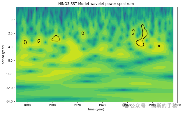
wave, period, scale, coi = wavelet(sst, dt, pad, dj, s0, j1, 'MORLET')
power = (np.abs(wave)) ** 2
# significance levels
signif = wave_signif(([1.0]), dt=dt, sigtest=0, scale=scale, lag1=0.72, mother='MORLET')
sig95 = signif[:, np.newaxis].dot(np.ones(n)[np.newaxis, :])
sig95 = power / sig95  # for > 1 values power is significant
​
# plot
plt.figure(figsize=(10, 6))
levels = np.array([2**i for i in range(-15,5)])
CS = plt.contourf(time, period, np.log2(power), len(levels))  #*** vagy 'contour'
im = plt.contourf(CS, levels=np.log2(levels))
plt.xlabel('time (year)')
plt.ylabel('period (year)')
plt.title('NINO3 SST Morlet wavelet power spectrum')
plt.xlim(xlim[:])
plt.yscale('log', base=2, subs=None)
plt.ylim([np.min(period), np.max(period)])
ax = plt.gca().yaxis
ax.set_major_formatter(matplotlib.ticker.ScalarFormatter())
plt.ticklabel_format(axis='y', style='plain')
plt.gca().invert_yaxis()
# 95% significance level
plt.contour(time, period, sig95, [-99, 1], colors='k')
plt.show()

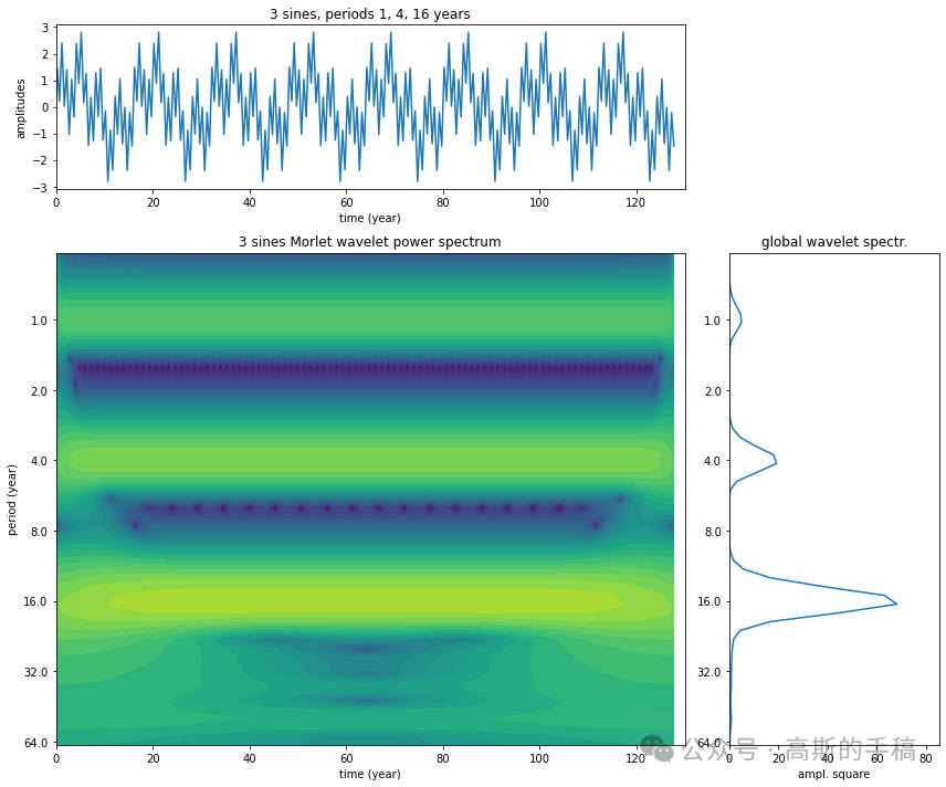
N = 512
dt = 0.25
t = np.arange(N) * dt
T1 = 1.0
T2 = 4.0
T3 = 16.0
w1 = 2 * np.pi / T1
w2 = 2 * np.pi / T2
w3 = 2 * np.pi / T3
s3 = np.sin(w1 * t) + np.sin(w2 * t) + np.sin(w3 * t)
​
pad = 1      # zero padding (recommended)
dj = 0.125   # 8 sub-octaves
s0 = 2*dt    # 6 month initial scale
j1 = 7/dj    # 7 octaves
mother = 'MORLET'  # mother wavelet
wave, period, scale, coi = wavelet(s3, dt, pad, dj, s0, j1, mother)
power = (np.abs(wave)) ** 2

Plot the signal and its wavelet spectrum:

variance = np.std(s3, ddof=1) ** 2
global_ws = variance * (np.sum(power, axis=1) / n)  # time-averaged global spectrum
​
from matplotlib import gridspec
gs = gridspec.GridSpec(2, 2, width_ratios=[3,1], height_ratios=[1,3])
​
#--- signal
xlim = ([0, 130])
plt.figure(figsize=(12, 10))
plt.subplot(gs[0,0])
plt.plot(t, s3)
plt.xlim(xlim[:])
plt.xlabel('time (year)')
plt.ylabel('amplitudes')
plt.title('3 sines, periods 1, 4, 16 years')
​
#--- wavelet power spectrum
plt3 = plt.subplot(gs[1,0])
levels = np.array([2**i for i in range(-18,10)])
CS = plt.contourf(t, period, np.log2(power), len(levels))  #*** or use 'contour'
im = plt.contourf(CS, levels=np.log2(levels))
plt.xlabel('time (year)')
plt.ylabel('period (year)')
plt.title('3 sines Morlet wavelet power spectrum')
plt.xlim(xlim[:])
# format y-scale
plt3.set_yscale('log', base=2, subs=None)
plt.ylim([np.min(period), np.max(period)])
ax = plt.gca().yaxis
ax.set_major_formatter(matplotlib.ticker.ScalarFormatter())
plt3.ticklabel_format(axis='y', style='plain')
plt3.invert_yaxis()
​
#--- global wavelet spectrum
plt4 = plt.subplot(gs[1,1])
plt.plot(global_ws, period)
plt.xlabel('ampl. square')
#plt.ylabel('period (year)')
plt.title('global wavelet spectr.')
plt.xlim([0, 1.25 * np.max(global_ws)])
# format y-scale
plt4.set_yscale('log', base=2, subs=None)
plt.ylim([np.min(period), np.max(period)])
ax = plt.gca().yaxis
ax.set_major_formatter(matplotlib.ticker.ScalarFormatter())
plt4.ticklabel_format(axis='y', style='plain')
plt4.invert_yaxis()
​
plt.tight_layout()
​
plt.show()

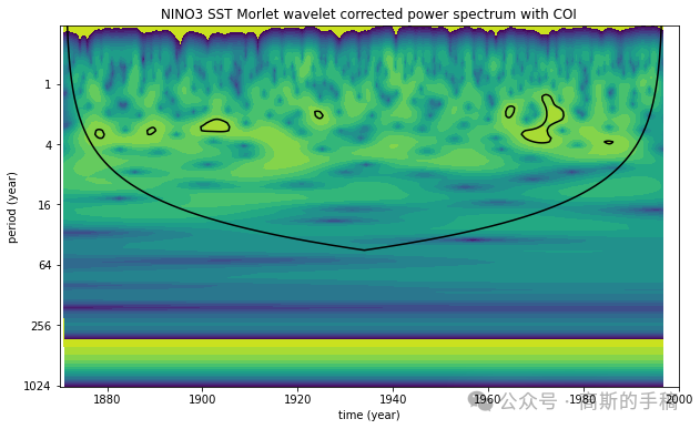
Cone of influence

n = len(sst)
dt = 0.25
time = np.arange(len(sst)) * dt + 1871.0  # array of time epochs
xlim = ([1870, 2000])
​
wave, period, scale, coi = wavelet(sst, dt, pad, dj, s0, j1, 'MORLET')
power = (np.abs(wave)) ** 2
# significance levels - calculated with uncorrected spectrum!
signif = wave_signif(([1.0]), dt=dt, sigtest=0, scale=scale, lag1=0.72, mother='MORLET')
sig95 = signif[:, np.newaxis].dot(np.ones(n)[np.newaxis, :])
sig95 = power / sig95  # power is significant where > 1
​
scale_ext = np.outer(scale,np.ones(n))
power = (np.abs(wave))**2 /scale_ext  # power spectrum (corrected)
​
# ábra
plt.figure(figsize=(10, 6))
levels = np.array([2**i for i in range(-15,5)])
CS = plt.contourf(time, period, np.log2(power), len(levels))  #*** or 'contour'
im = plt.contourf(CS, levels=np.log2(levels))
plt.xlabel('time (year)')
plt.ylabel('period (year)')
plt.title('NINO3 SST Morlet wavelet corrected power spectrum with COI')
plt.xlim(xlim[:])
plt.yscale('log', base=2, subs=None)
plt.ylim([np.min(period), np.max(period)])
ax = plt.gca().yaxis
ax.set_major_formatter(matplotlib.ticker.ScalarFormatter())
plt.ticklabel_format(axis='y', style='plain')
plt.gca().invert_yaxis()
# 95% significance level
plt.contour(time, period, sig95, [-99, 1], colors='k')
# Cone of influence (COI)
plt.plot(time, coi[:-1], 'k')
plt.show()

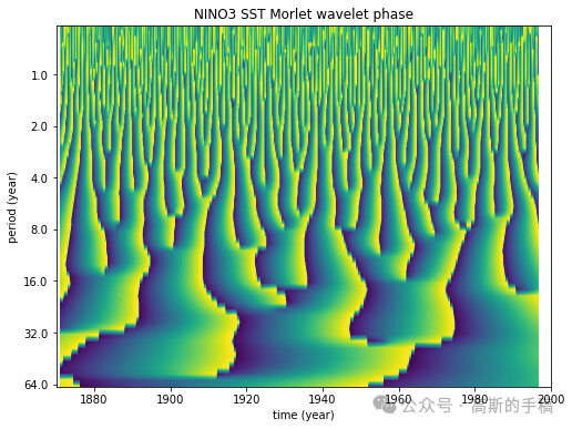
Phase

phase = (np.angle(wave))
​
plt.figure(figsize=(8, 6))
levels = np.arange(-np.pi,np.pi,0.1)
CS = plt.contourf(time, period, phase, len(levels))  #*** or 'contour'
im = plt.contourf(CS, levels=levels)
plt.xlabel('time (year)')
plt.ylabel('period (year)')
plt.title('NINO3 SST Morlet wavelet phase')
plt.xlim(xlim[:])
plt.yscale('log', base=2, subs=None)
plt.ylim([np.min(period), np.max(period)])
ax = plt.gca().yaxis
ax.set_major_formatter(matplotlib.ticker.ScalarFormatter())
plt.ticklabel_format(axis='y', style='plain')
plt.gca().invert_yaxis()
plt.show()

完整代码可通过学术咨询获得：