


引言:为什么需要两阶段法?
在解决线性规划问题时,单纯形法要求初始基可行解必须存在。然而,现实中的许多问题(如资源分配、生产计划)的约束条件可能不包含现成的单位矩阵,导致无法直接启动算法。两阶段法(Two-Phase Method)通过引入人工变量分阶段处理这一问题,成为运筹学中解决无初始可行基问题的核心工具。本文将从理论推导到代码实现解析这一方法。
一、两阶段法的数学原理与步骤分解
1. 第一阶段:构造辅助问题消除人工变量
- 目标:通过最小化人工变量的和,找到原问题的初始可行基
- 操作:将原目标系数暂时取零值。根据最优解的判别定理和改进的基可行解方法进行基的转换,使得人工变量逐渐换出基底
- 数学模型:
- 原问题 :
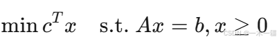
- 原问题阶段Ⅰ :
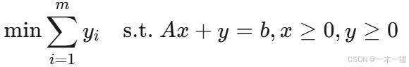
- 原问题 :
- 终止条件:
- 若最优值 > 0 → 原问题无解
- 若最优值 = 0 → 剔除人工变量,进入阶段Ⅱ
2. 第二阶段:求解原问题
- 目标:利用阶段Ⅰ得到的基变量,构建修正单纯形表,执行标准单纯形法迭代
- 操作:再丢掉人工变量对应的列,恢复原线性规划问题的目标系数,寻找原问题的最优解
注意:推荐可深入了解单纯性法再阅读此文。可阅读下文了解单纯形法!(运筹学之单纯形法(超详细讲解 + matlab可运行代码实现)-CSDN博客)
二、与大M法的对比:优劣分析
| 对比维度 | 两阶段法 | 大M法 |
|---|---|---|
| 数值稳定性 | 避免大常数M导致的舍入误差 | M值选取不当易引发计算错误 |
| 实现复杂度 | 需分阶段实现,代码结构清晰 | 单阶段但需处理混合系数 |
| 适用场景 | 人工变量较多的问题 | 人工变量较少的小规模问题 |
三、案例分析
案例背景:电子产品生产优化
某工厂生产两种智能手表(型号A和B),需优化日产量以最大化利润。已知:
- 资源约束:
- 芯片供应:每生产1个A消耗2个芯片,1个B消耗3个芯片,每日芯片总量≤1200个
- 组装工时:A需4小时,B需3小时,每日总工时≤800小时
- 包装限制:每日最多可包装300个A或250个B(非线性约束线性化后:
x_A ≤ 300,x_B ≤ 250)
- 市场需求:A至少生产100个(
x_A ≥ 100) - 利润目标:A每个利润¥150,B¥200
3.1 数学建模与标准化
3.1.1 原问题标准形(最大化→最小化)
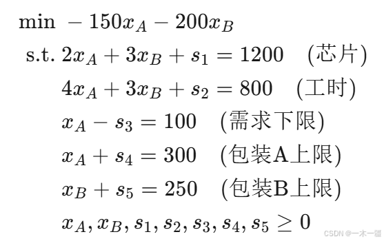
注:需求约束 x_A ≥ 100 引入人工变量 a_1,需使用两阶段法。
3.2 两阶段法分步计算
阶段Ⅰ:构造辅助问题消除人工变量
- 目标函数:
min a1 - 约束:
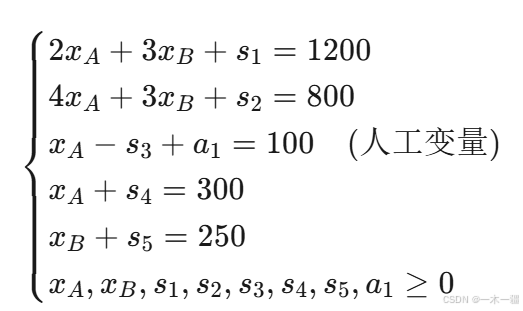
- 求解结果:最优值=0 → 存在可行解,人工变量
a1=0,初始基为{s1, s2, a1, s4, s5}
阶段Ⅱ:求解原问题
- 目标函数:
min -150x_A -200x_B - 初始基:
{s1, s2, x_A, s4, s5}(剔除人工变量) - 最终解:
x_A=100, x_B=200, s1=200, s4=200, s5=50→ 最大利润=150×100 +200×200=55,000元
四、用Python实现两阶段法
以上述案例为例,有需要请自行调整。
import numpy as np

def enhanced_simplex(c, A, b, max_iter=500, tol=1e-8):
    """
    Enhanced simplex method with two-phase approach.

    Inputs:
        c : np.ndarray - Objective function coefficients (n×1)
        A : np.ndarray - Constraint matrix (m×n)
        b : np.ndarray - Right-hand-side constants (m×1)
        max_iter : int - Maximum number of iterations (default: 500)
        tol : float - Tolerance for numerical precision (default: 1e-8)

    Outputs:
        xm : np.ndarray - Optimal solution
        fm : float - Optimal objective value
        status : int - Solver status flag (1 = optimal, 0 = unbounded, -1 = infeasible)
        iterations : int - Number of iterations performed
    """
    # Dimensions
    m, n = A.shape

    # Phase 1: Artificial problem setup
    phase1_A = np.hstack((A, np.eye(m)))  # Append artificial variables
    phase1_c = np.hstack((np.zeros(n), np.ones(m)))  # Objective function for Phase 1

    # Initial basic variables: artificial variables
    initial_basis = list(range(n, n + m))

    # Solve artificial problem
    x_phase1, _, status, _ = simplex_core(phase1_A, phase1_c, b, initial_basis, max_iter, tol)

    if status != 1 or np.any(x_phase1[n:] > tol):
        print("No feasible solution: Phase 1 failed.")
        return None, None, -1, 0

    # Phase 2: Solve original problem
    basis = [i for i in range(n) if x_phase1[i] > tol]
    xm, fm, status, iterations = simplex_core(A, c, b, basis, max_iter, tol)

    return xm, fm, status, iterations


def simplex_core(A, c, b, basis, max_iter=1000, tol=1e-8):
    """
    Core simplex solver for a single phase.

    Inputs:
        A : np.ndarray - Constraint matrix (m×n)
        c : np.ndarray - Objective function coefficients
        b : np.ndarray - Right-hand-side constants
        basis : list - Initial basic variable indices
        max_iter : int - Maximum number of iterations (default: 1000)
        tol : float - Tolerance for numerical precision (default: 1e-8)

    Outputs:
        x : np.ndarray - Optimal solution
        fval : float - Optimal objective value
        status : int - Solver status flag (1 = optimal, 0 = unbounded, -1 = iteration limit reached)
        iterations : int - Number of iterations performed
    """
    m, n = A.shape
    x = np.zeros(n)
    iterations = 0

    # Check initial basis is valid
    B = A[:, basis]
    if np.linalg.matrix_rank(B) < m:
        raise ValueError("Initial basis matrix is not full rank.")

    for iterations in range(1, max_iter + 1):
        # Solve for basic variables
        B_inv = np.linalg.inv(B)
        x_b = B_inv @ b
        x[basis] = x_b

        # Compute reduced costs
        c_B = c[basis]
        y = c_B @ B_inv
        reduced_costs = c - y @ A

        # Check for optimality
        if np.all(reduced_costs >= -tol):
            fval = c @ x
            return x, fval, 1, iterations

        # Identify entering variable (most negative reduced cost)
        q = np.argmin(reduced_costs)

        # Compute direction d
        d = B_inv @ A[:, q]
        if np.all(d <= tol):
            # If all entries in d are non-positive, problem is unbounded
            return None, None, 0, iterations

        # Compute theta (ratio test)
        theta = np.full(m, np.inf)
        for i in range(m):
            if d[i] > tol:
                theta[i] = x_b[i] / d[i]

        # Identify leaving variable
        p = np.argmin(theta)
        if theta[p] == np.inf:
            return None, None, 0, iterations

        # Update basis
        basis[p] = q
        B = A[:, basis]

    # If maximum iterations reached
    return None, None, -1, iterations


# Example usage
if __name__ == "__main__":
    # Example problem
    c = np.array([-150, -200, 0, 0, 0, 0, 0])
    A = np.array([
        [2, 3, 1, 0, 0, 0, 0],
        [4, 3, 0, 1, 0, 0, 0],
        [1, 0, 0, 0, -1, 0, 0],
        [1, 0, 0, 0, 0, 1, 0],
        [0, 1, 0, 0, 0, 0, 1]
    ])
    b = np.array([1200, 800, 100, 300, 250])

    xm, fm, status, iterations = enhanced_simplex(c, A, b)

    if status == 1:
        print("Optimal solution:")
        print(xm)
        print(f"Optimal objective value: {fm}")
    elif status == 0:
        print("Problem is unbounded.")
    else:
        print("No feasible solution or iteration limit reached.")
如有问题,可私信或在评论区交流,定即时回复,感谢支持!


 6725
6725

 被折叠的 条评论
为什么被折叠?
被折叠的 条评论
为什么被折叠?
 到【灌水乐园】发言


