深度学习进阶：自然语言处理入门：第三章

深度学习进阶：自然语言处理入门：第三章Wordvec

本章主题：单词分布式的表示

上一章回顾：使用计数法得到单词的分布式

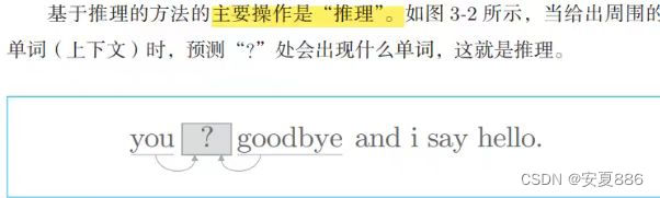
本章核心：讨论该方法的替代方法－－基于推理的方法

热点：推理机制：神经网络

著名的Wordvec登场（实现的为简单的Wordvec,所以会牺牲一定的效率， 但是如果不用它处理大规模数据，处理些许小数据还是绰绰有余的嘞）

3.1.1 基于计数的方法的问题

基于计数的方法使用整个语料库的统计数据（共现矩阵和 PPMI 等）， 通过一次处理（SVD 等）获得单词的分布式表示。而基于推理的方法使用 神经网络，通常在 mini-batch 数据上进行学习。这意味着神经网络一次只 需要看一部分学习数据（mini-batch），并反复更新权重。
​ 基于计数的方法一次性处理全部学习数据；反之，基于推理的方法使用部分学习数据逐步学习。
使用了共现矩阵和PPMI等
拓：
共现矩阵：统计文本中两两词组之间共同出现的次数，以此来描述词组间的亲密度，看他们关系好不好的呢。
代码实现：

import sys
sys.path.append('..')
import numpy as np
from common.util import preprocess
text = 'You say goodbye and I say hello.'
corpus, word_to_id, id_to_word = preprocess(text)
print(corpus)
# [0 1 2 3 4 1 5 6]
print(id_to_word)
# {0: 'you', 1: 'say', 2: 'goodbye', 3: 'and', 4: 'i', 5: 'hello', 6: '.'}

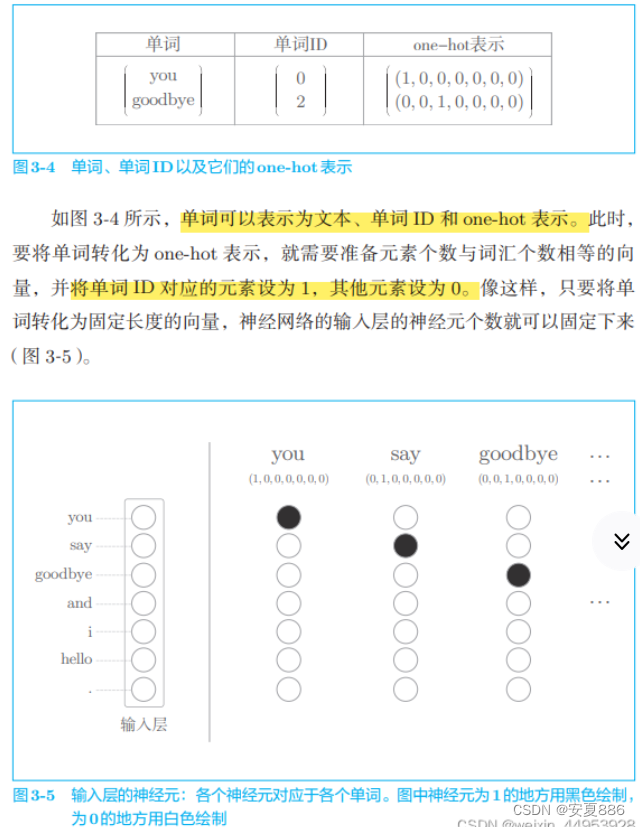
从下文图片可看出，单词you的上下文仅仅只 有say这个单词。

所以呢，用表格表示的话，就是下图，之后我们会将下表的数字用作我们单词信息查询坐标的，所以这是有用的嘞。
比如说：我们可以用向量[0, 1, 0, 0, 0, 0, 0]来表示单词you

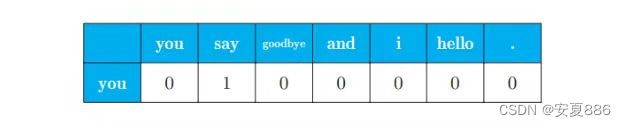
向量此时可以理解成you的位置坐标
如果此时我们将上面全部的单词实现上述操作，就会得到下图：

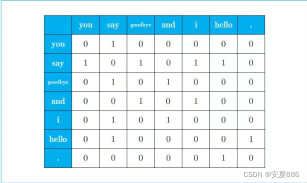
上图呢，就是汇总了所有单词的共现单词的表格，这个表格记录了每个单词的位置，专业术语将它说成是向量。因为上面这个表格是矩形的形状，然后呢，将所有单词的位置呈现出来了的，因此，有位大牛就把它称为共现矩阵（英文或者代码中，我们把共现矩阵命名为：co-occurence-matrix)
共现矩阵代码实现：

C = np.array([
 [0, 1, 0, 0, 0, 0, 0],
 [1, 0, 1, 0, 1, 1, 0],
 [0, 1, 0, 1, 0, 0, 0],
 [0, 0, 1, 0, 1, 0, 0],
 [0, 1, 0, 1, 0, 0, 0],
 [0, 1, 0, 0, 0, 0, 1],
 [0, 0, 0, 0, 0, 1, 0],
], dtype=np.int32)
print(C[0]) # 单词ID为0的向量
# [0 1 0 0 0 0 0]
print(C[4]) # 单词ID为4的向量
# [0 1 0 1 0 0 0]
print(C[word_to_id['goodbye']]) # goodbye的向量
# [0 1 0 1 0 0 0]
共现矩阵的函数: 
create_co_matrix(corpus, vocab_size, window_size=1)
其中参数 corpus 是单词 ID 列表
参数 vocab_ size 是词汇个数
window_size 是窗口大小
代码实现：
def create_co_matrix(corpus, vocab_size, window_size=1):
    '''生成共现矩阵
    :param corpus: 语料库（单词ID列表）
    :param vocab_size:词汇个数，重复的单词算成一个
    :param window_size:窗口大小（当窗口大小为1时，左右各1个单词为上下文）
    :return: 共现矩阵
    '''
    corpus_size = len(corpus)        #单词总数，包括重度的单词
    co_matrix = np.zeros((vocab_size, vocab_size), dtype=np.int32)
    for idx, word_id in enumerate(corpus):
        for i in range(1, window_size + 1):
            left_idx = idx - i
            right_idx = idx + i
            if left_idx >= 0:
                left_word_id = corpus[left_idx]
                co_matrix[word_id, left_word_id] += 1
            if right_idx < corpus_size:
                right_word_id = corpus[right_idx]
                co_matrix[word_id, right_word_id] += 1
    return co_matrix

 

拓：
PPMI: 可以改进共现矩阵

共现矩阵的缺陷：

共现矩阵的元素表示两个单词同时出现的次数，这里的次数并不具备好的性质，举个例子，有短语叫the car，因为the是个常用词，如果以两个单词同时出现的次数为衡量相关性的标准，与drive 相比，the和car的相关性更强，这是不对的。

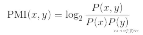
PMI（简单称呼为：点互信息）介绍：

点互信息(Pointwise Mutual Information,PMI)：表达式如下，P(x)表示x发生的概率，P(y)表示y发生的概率，P(x,y)表示x和y同时发生的概率。PMI的值越高，表明x与y相关性越强。
通俗讲，PMI就是求两个事件同时发生的概率有多大，他们发生的概率越大，则PMI的值就越大的嘞，也就表示两个事件的关联性就越强，放在男女之间，就说明她和他的关系就越亲密的呢，就好比令人神往的青梅竹马，流口水哇，小编也想要哇（努力加油哇！）。
下图是数学原理图：

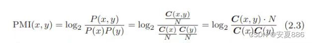
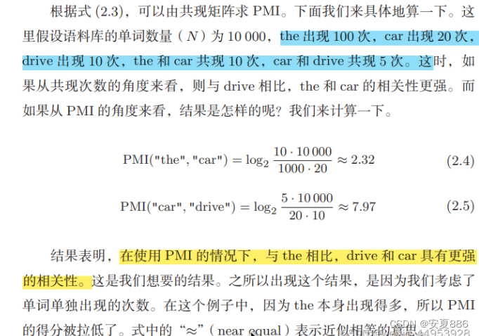
由此可见，点互信息可以帮助我们将the和car的相关性降低，并且提高drive和car的相关性，从而修正出我们想要的结果。
但是，如果两个单词的共现次数为0时，就会出现log₂0 = -∞
的尴尬，为了解决这个奇葩，所以我们采用正的点互信息，
见名知意，就是只是用正的数据，不会使用负数，PPMI可以将负数转化成0，这样就可以轻松的处理掉这个奇葩啦！

PPMI：（正的点互信息）

正点互信息只是比点互信息多了一个判断最大值的操作，小于0的值都改成了0
共现矩阵转化成PPMI矩阵的函数代码实现：

def ppmi(C, verbose=False, eps = 1e-8):
    '''生成PPMI（正的点互信息）
    :param C: 共现矩阵
    :param verbose: 是否输出进展情况
    :return:
    '''
    M = np.zeros_like(C, dtype=np.float32)
    N = np.sum(C)
    S = np.sum(C, axis=0)
    total = C.shape[0] * C.shape[1]
    cnt = 0
    for i in range(C.shape[0]):
        for j in range(C.shape[1]):
            pmi = np.log2(C[i, j] * N / (S[j]*S[i]) + eps)
            M[i, j] = max(0, pmi)
            if verbose:
                cnt += 1
                if cnt % (total//100 + 1) == 0:
                    print('%.1f%% done' % (100*cnt/total))
    return M

注解：
verbose 是决定是否输出运行情况的标志
当处理大语料库时，设置 verbose=True，可以用于确认运行情况。在这段代码 中，为了仅从共现矩阵求 PPMI 矩阵而进行了简单的实现。

设置共现矩阵代码：

import numpy as np
C = np.array([
 [0, 1, 0, 0, 0, 0, 1],
 [1, 0, 1, 0, 1, 1, 0],
 [0, 1, 0, 1, 0, 0, 0],
 [0, 0, 1, 0, 1, 0, 0],
 [0, 1, 0, 1, 0, 0, 0],
 [0, 1, 0, 0, 0, 0, 1],
 [0, 0, 0, 0, 0, 1, 0],
], dtype=np.int32)
N = np.sum(C)  #15
S = np.sum(C, axis=0) #array([1, 4, 2, 2, 2, 2, 2])

执行函数代码：

import sys
sys.path.append('..')
import numpy as np
from common.util import preprocess, create_co_matrix, cos_similarity, ppmi
text = 'You say goodbye and I say hello.'
corpus, word_to_id, id_to_word = preprocess(text)
vocab_size = len(word_to_id)
C = create_co_matrix(corpus, vocab_size)
W = ppmi(C)
np.set_printoptions(precision=3)  # 有效位数为3位
print('covariance matrix')
print(C)
print('-'*50)
print('PPMI')
print(W)
输出结果：
covariance matrix
[[0 1 0 0 0 0 0]
 [1 0 1 0 1 1 0]
 [0 1 0 1 0 0 0]
 [0 0 1 0 1 0 0]
 [0 1 0 1 0 0 0]
 [0 1 0 0 0 0 1]
 [0 0 0 0 0 1 0]]
--------------------------------------------------
PPMI
[[0.    1.807 0.    0.    0.    0.    0.   ]
 [1.807 0.    0.807 0.    0.807 0.807 0.   ]
 [0.    0.807 0.    1.807 0.    0.    0.   ]
 [0.    0.    1.807 0.    1.807 0.    0.   ]
 [0.    0.807 0.    1.807 0.    0.    0.   ]
 [0.    0.807 0.    0.    0.    0.    2.807]
 [0.    0.    0.    0.    0.    2.807 0.   ]]
Process finished with exit code 0

总结：

优点：

PPMI 矩 阵的各个元素均为大于等于 0 的实数。我们得到了一个由更好的指标形成的 矩阵，这相当于获取了一个更好的单词向量。

缺陷：

但是，这个 PPMI 矩阵还是存在一个很大的问题，那就是随着语料库 的词汇量增加，各个单词向量的维数也会增加。如果语料库的词汇量达到 10 万，则单词向量的维数也同样会达到 10 万。实际上，处理 10 万维向量 是不现实的。
降维
所谓降维，就是将高维转化为低维，将复杂的数据转换为简单的数据，目的就是将问题简单化，将价值低的数据筛选处理掉，保留重要信息，简称：去其糟粕，取其精华。
实例：
向量中的大多数元素为 0 的矩阵（或向量）称为稀疏矩阵（或稀疏向 量）。这里的重点是，从稀疏向量中找出重要的轴，用更少的维度对 其进行重新表示。结果，稀疏矩阵就会被转化为大多数元素均不为 0 的密集矩阵。这个密集矩阵就是我们想要的单词的分布式表示。
图例：

SVD:奇异值分解

接下来，我们使用 Python 来实现 SVD，这里可以使用 NumPy 的 linalg 模块中的 svd 方法。
linalg 是 linear algebra（线性代数）的简称。（下方代码会用到）
下 面，我们创建一个共现矩阵，将其转化为 PPMI 矩阵，然后对其进行 SVD

import sys
sys.path.append('..')
import numpy as np
import matplotlib.pyplot as plt
from common.util import preprocess, create_co_matrix, ppmi
text = 'You say goodbye and I say hello.'
corpus, word_to_id, id_to_word = preprocess(text)
vocab_size = len(id_to_word)
C = create_co_matrix(corpus, vocab_size, window_size=1)
W = ppmi(C)
# SVD
U, S, V = np.linalg.svd(W)
np.set_printoptions(precision=3)  # 有效位数为3位
 # 共现矩阵
print(C[0])        # [0 1 0 0 0 0 0]
 # PPMI矩阵
print(W[0])        #[0.    1.807 0.    0.    0.    0.    0.   ]
# SVD
print(U[0])    #[-3.409e-01 -1.110e-16 -3.886e-16 -1.205e-01  0.000e+00  9.323e-012.226e-16]
# plot
for word, word_id in word_to_id.items():
    plt.annotate(word, (U[word_id, 0], U[word_id, 1]))
plt.scatter(U[:,0], U[:,1], alpha=0.5)
plt.show()

结论：

原先的稀疏向量 W[0] 经过 SVD 被转化成了密集向量 U[0]。如果要对这个密集向量降维，比如把它降维到二维向量，取出前两个元素 即可。
代码观测：

print(U[0, :2])
# [ 3.409e-01 -1.110e-16]

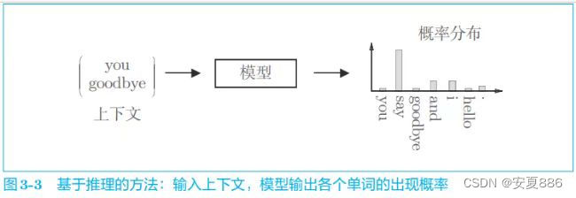
3.1.2  基于推理的方法概要

推理模型出现概率统计：

3.1.3  神经网络中的单词处理的方法

最终得出结论：
用向量表示单词具体位置的哈

3.2 简单的wordvec

Wordvec:最初指程序或者工具
但随着时代发展，某些情况下也指：神经网络模型
具体点，是指CBOW模型和skip-gram模型的神经网络

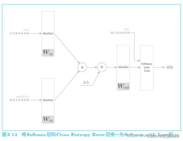
3.2.1  CBOW模型的推理

总的来说，CBOW模型就是一个可以根据上下文预测单词的神经网络的哈。（是不是有点类似英语那神秘莫测的语感，高中时，英语语感做题，不就是凭借上下文来轻松选出正确选项吗？不是类似，而是神似呢）

上面的灰度最深的部分就是与you和goodbye都共同拥有的概率最大的单词啦

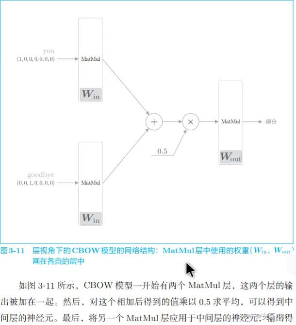
CBOW代码实现：

# coding: utf-8
import sys
sys.path.append('..')
import numpy as np
from common.layers import MatMul
# 样本的上下文数据
c0 = np.array([[1, 0, 0, 0, 0, 0, 0]])
c1 = np.array([[0, 0, 1, 0, 0, 0, 0]])
# 初始化权重
W_in = np.random.randn(7, 3)
W_out = np.random.randn(3, 7)
# 生成层
in_layer0 = MatMul(W_in)
in_layer1 = MatMul(W_in)
out_layer = MatMul(W_out)
# 正向传播
h0 = in_layer0.forward(c0)
h1 = in_layer1.forward(c1)
h = 0.5 * (h0 + h1)
s = out_layer.forward(h)
print(s)
# [[-0.33304998  3.19700011  1.75226542  1.36880744  1.68725368  2.38521564 0.81187955]]

CBOW 模型的学习就是调整权重，以使预测准确。其结果是，权重 Win（确切地说是 Win 和 Wout 两者）学习到蕴含单词出现模式的向量。根据过去的实验，CBOW 模型（和 skip-gram 模型）得到的单词的分布式表示，特别是使用维基百科等大规模语料库学习到的单词的分布式表示，在单词的含义和语法上符合我们直觉的案例有很多.
CBOW模型只是学习语料库中单词的出现模式。如果语料库不一样， 学习到的单词的分布式表示也不一样。比如，只使用“体育”相关 的文章得到的单词的分布式表示，和只使用“音乐”相关的文章得 到的单词的分布式表示将有很大不同。
结论：CBOW学习到内容并不一定可以适用于全部数据，例如从游戏语言和音乐语言，它们学习到的数据就有可能有很大的不同，比如可能会出现：预测的正确率下降的嘞。

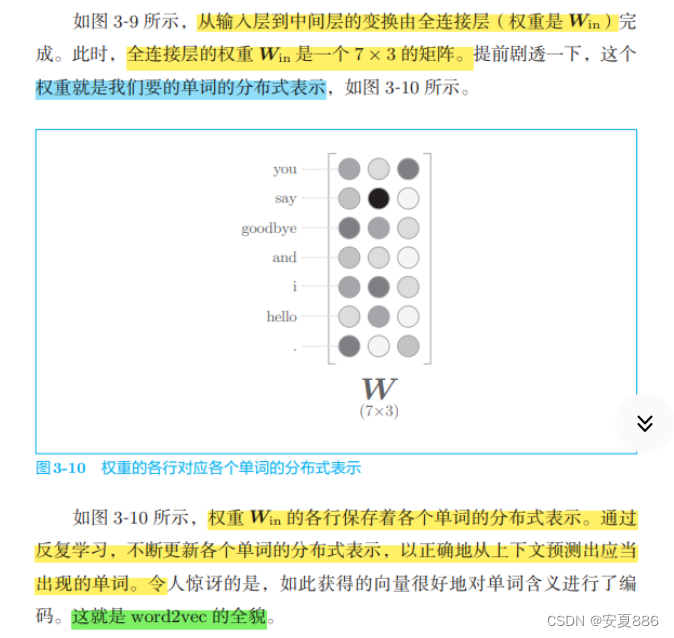
3.2.3 Word2vec的权重和分布式表示

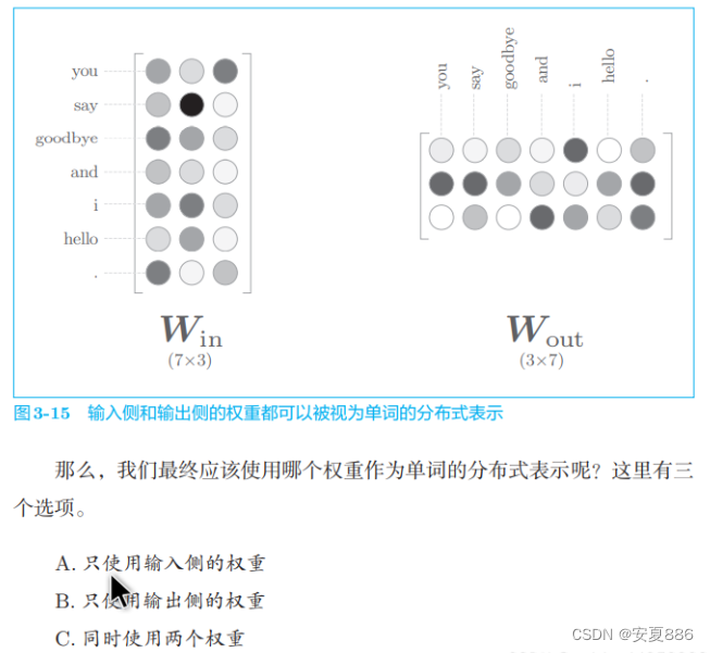
就 word2vec（特别是 skip-gram 模型）而言，最受欢迎的是方案 A。遵循这一思路，我们也使用 Win 作为单词的分布式表示
个人理解：我认为是原汁原味的原因，所以选择了A的，因为输出的数据是综合的两个数据的平均，所以可能对原始数据有所破坏的嘞！

3.3 学习数据的准备

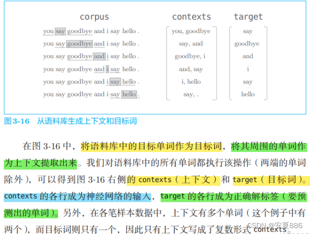
在开始 word2vec 的学习之前，我们先来准备学习用的数据。这里我们 仍以“You say goodbye and I say hello.”这个只有一句话的语料库为例进 行说明。

3.3.1 上下文和目标词

word2vec 中使用的神经网络的输入是上下文，它的正确解标签是被这些上下文包围在中间的单词，即目标词。
通俗点，就是要凭借机器语感预测的神秘单词。

def preprocess(text):
    text = text.lower()
    text = text.replace('.', ' .')
    words = text.split(' ')
    word_to_id = {}
    id_to_word = {}
    for word in words:
        if word not in word_to_id:
            new_id = len(word_to_id)
            word_to_id[word] = new_id
            id_to_word[new_id] = word
    corpus = np.array([word_to_id[w] for w in words])
    return corpus, word_to_id, id_to_word

我们来实现从语料库生成上下文和目标词的函数。在此之前，我 们可以用上一章学到的内容。首先，将语料库的文本转化成单词 ID。

代码实现：

import sys
sys.path.append('..')
from common.util import preprocess
text = 'You say goodbye and I say hello.'
corpus, word_to_id, id_to_word = preprocess(text)
print(corpus)
# [0 1 2 3 4 1 5 6]
print(id_to_word)
# {0: 'you', 1: 'say', 2: 'goodbye', 3: 'and', 4: 'i', 5: 'hello', 6: '.'}

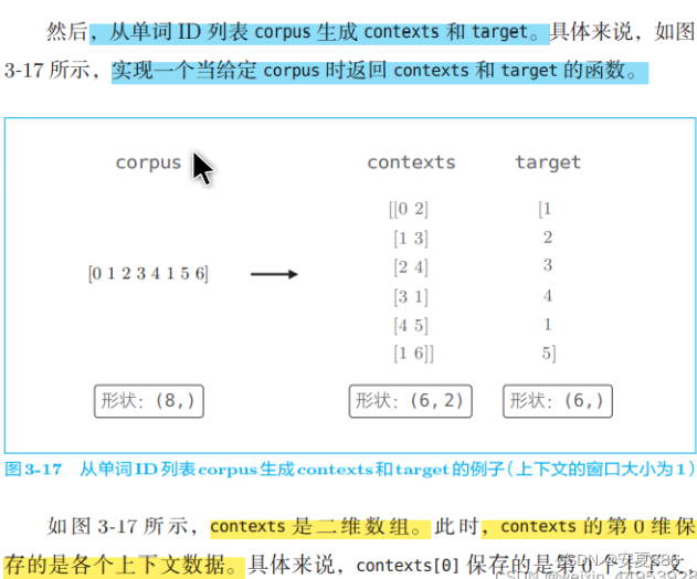
生成上下文和目标词的函数

create_contexts_target(corpus, window_size)

def create_contexts_target(corpus, window_size=1):
    '''生成上下文和目标词
    :param corpus: 语料库（单词ID列表）
    :param window_size: 窗口大小（当窗口大小为1时，左右各1个单词为上下文）
    :return:
    '''
    target = corpus[window_size:-window_size]
    contexts = []
    for idx in range(window_size, len(corpus)-window_size):
        cs = []
        for t in range(-window_size, window_size + 1):
            if t == 0:
                continue
            cs.append(corpus[idx + t])
        contexts.append(cs)
    return np.array(contexts), np.array(target)
contexts, target = create_contexts_target(corpus, window_size=1)
print(contexts)
# [[0 2]
# [1 3]
# [2 4]
# [3 1]
# [4 5]
# [1 6]]
print(target)
# [1 2 3 4 1 5]

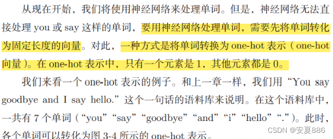
3.3.2  转化为one-hot表示

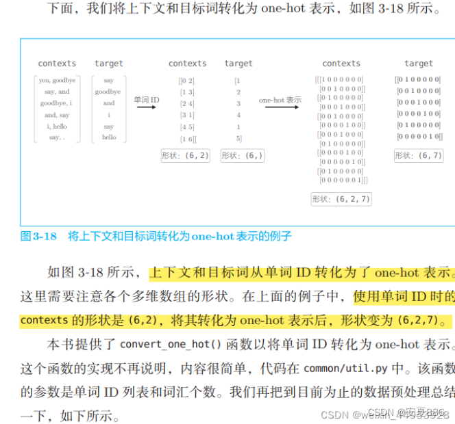
理解：（6，2，7）是6行2列然后最里面的中括号里面有七个元素
2也可以理解为是2维的意思的呢，啥是2维得嘞？通俗点，就是中括号的数量的嘞，（目前这样理解，可能原理不对，但能明白其含义的）
转化为one-hot的代码实现：

def convert_one_hot(corpus, vocab_size):
    '''转换为one-hot表示
    :param corpus: 单词ID列表（一维或二维的NumPy数组）
    :param vocab_size: 词汇个数
    :return: one-hot表示（二维或三维的NumPy数组）
    '''
    N = corpus.shape[0]
    if corpus.ndim == 1:
        one_hot = np.zeros((N, vocab_size), dtype=np.int32)
        for idx, word_id in enumerate(corpus):
            one_hot[idx, word_id] = 1
    elif corpus.ndim == 2:
        C = corpus.shape[1]
        one_hot = np.zeros((N, C, vocab_size), dtype=np.int32)
        for idx_0, word_ids in enumerate(corpus):
            for idx_1, word_id in enumerate(word_ids):
                one_hot[idx_0, idx_1, word_id] = 1
    return one_hot

实现代码如下，（完成了这个，机器学习数据的准备就完成了的，轻松哇）

text = 'You say goodbye and I say hello.'
corpus, word_to_id, id_to_word = preprocess(text)
contexts, target = create_contexts_target(corpus, window_size=1)
vocab_size = len(word_to_id)
target = convert_one_hot(target, vocab_size)
contexts = convert_one_hot(contexts, vocab_size)
contexts
#输出contexts
array([[[1, 0, 0, 0, 0, 0, 0],
        [0, 0, 1, 0, 0, 0, 0]],
       [[0, 1, 0, 0, 0, 0, 0],
        [0, 0, 0, 1, 0, 0, 0]],
       [[0, 0, 1, 0, 0, 0, 0],
        [0, 0, 0, 0, 1, 0, 0]],
       [[0, 0, 0, 1, 0, 0, 0],
        [0, 1, 0, 0, 0, 0, 0]],
       [[0, 0, 0, 0, 1, 0, 0],
        [0, 0, 0, 0, 0, 1, 0]],
       [[0, 1, 0, 0, 0, 0, 0],
        [0, 0, 0, 0, 0, 0, 1]]])

3.4 CBOW模型的实现

原理图：

简单的CBOW的代码实现：

这里，我们假定参数 contexts 是一个三维 NumPy 数组，即上一节图 3-18 的例子中 (6,2,7)的形状，其中第 0 维的元素个数是 mini-batch 的数量， 第 1 维的元素个数是上下文的窗口大小，第 2 维表示 one-hot 向量。此外， target 是 (6,7) 这样的二维形状。
 

class SimpleCBOW:
    def __init__(self, vocab_size, hidden_size):
        V, H = vocab_size, hidden_size        #词汇个数 vocab_size,中间层的神经元个数 hidden_size
        # 初始化权重,并用一些小的随机值初始化这两个权重,astype('f')初始化将使用 32 位的浮点数。
        W_in = 0.01 * np.random.randn(V, H).astype('f')
        W_out = 0.01 * np.random.randn(H, V).astype('f')
        # 生成层
        #生成两个输入侧的 MatMul 层、一个输出侧的 MatMul 层，以及一个 Softmax with Loss 层。
        self.in_layer0 = MatMul(W_in)
        self.in_layer1 = MatMul(W_in)
        self.out_layer = MatMul(W_out)
        self.loss_layer = SoftmaxWithLoss()
        # 将所有的权重和梯度整理到列表中
        layers = [self.in_layer0, self.in_layer1, self.out_layer]
        self.params, self.grads = [], []
        for layer in layers:
            self.params += layer.params
            self.grads += layer.grads
        # 将单词的分布式表示设置为成员变量
        self.word_vecs = W_in
    #现神经网络的正向传播 forward() 函数
    def forward(self, contexts, target):
        h0 = self.in_layer0.forward(contexts[:, 0])
        h1 = self.in_layer1.forward(contexts[:, 1])
        h = (h0 + h1) * 0.5
        score = self.out_layer.forward(h)
        loss = self.loss_layer.forward(score, target)
        return loss
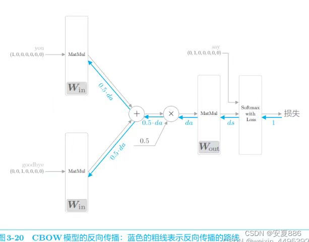
    def backward(self, dout=1):
        ds = self.loss_layer.backward(dout)
        da = self.out_layer.backward(ds)
        da *= 0.5
        self.in_layer1.backward(da)
        self.in_layer0.backward(da)
        return None

庆祝，反向传播的实现至此就结束啦!

我们已经将各个权重参数的梯度保存在了变量：grads中啦
然后呢，先调用forward()函数,再调用backward()函数，grads列表中的梯度就会被更新啦！
接下来，再看看SimpleCBOW类的学习
学习的实现：
（使用的还是第一章所用到的Trainer）

import sys
sys.path.append('..')  # 为了引入父目录的文件而进行的设定
from common.trainer import Trainer
from common.optimizer import Adam
from simple_cbow import SimpleCBOW
from common.util import preprocess, create_contexts_target, convert_one_hot
window_size = 1
hidden_size = 5
batch_size = 3
max_epoch = 1000
text = 'You say goodbye and I say hello.'
corpus, word_to_id, id_to_word = preprocess(text)
vocab_size = len(word_to_id)
contexts, target = create_contexts_target(corpus, window_size)
target = convert_one_hot(target, vocab_size)
contexts = convert_one_hot(contexts, vocab_size)
model = SimpleCBOW(vocab_size, hidden_size)
optimizer = Adam()
trainer = Trainer(model, optimizer)
trainer.fit(contexts, target, max_epoch, batch_size)
trainer.plot()
word_vecs = model.word_vecs  #为输入侧的 MatMul 层的权重已经赋值给了成员变量 word_vecs
for word_id, word in id_to_word.items():
    print(word, word_vecs[word_id])

学习结果：

you [ 1.1550112  1.2552509 -1.1116056  1.1482503 -1.2046812]
say [-1.2141827  -1.2367412   1.2163384  -1.2366292   0.67279905]
goodbye [ 0.7116186   0.55987084 -0.8319744   0.749239   -0.8436555 ]
and [-0.94652086 -0.8535852   0.55927175 -0.6934891   2.0411916 ]
i [ 0.7177702  0.5699475 -0.8368816  0.7513028 -0.8419596]
hello [ 1.1411363  1.2600429 -1.105042   1.1401148 -1.2044929]
. [-1.1948084 -1.2921802  1.4119368 -1.345656  -1.5299033]

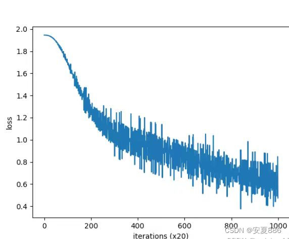
由图可知：从咱们小型的语料库中进行实现，效果并不好的，为啥子？你看哇，纵轴的loss虽然降低啦，但是你再看看波动率，是真的很大哇，你愿意和一个忽冷忽热的伴侣在一起吗？不愿意哇！这个也是如此
当 然，主要原因是语料库太小了。如果换成更大、更实用的语料库，相信会获 得更好的结果。
但是，还有一个不足：
处理的效率太低了，速度真的很慢很慢的嘞。
等待，无意等于谋财害命，这是赤裸裸的慢性自杀！
所以呢，我们可以完善改进一下这个简单的CBOW模型，让它变成一个真正的"CBOW".(放飞烦恼。做真正的自己！)
如何见证CBOW做回自己，敬请期待下一章节娓娓道来！

拓展：

skip-gram模型简单叙述：它其实就是CBOW的反转，也是这位兄弟的互补，它比CBOW更加强大，因为，它是通过自己一个单词预测它周围的单词的嘞（挠挠小脑袋，这不就是搜狗输入法的语句联想功能嘛！
比如：我输入“我爱”，输入法就会根据我经常输入的内容，联想到周围的词汇:"这家伙莫非又是向那位倾慕已久的姑娘表白？好吧，看我的智能联想，给主人脑补下一句，哈哈，我可真聪明哇！"）