


本文旨在深入探究影响广州市二手房房价变化的各类因素,并通过构建有效的预测模型,为相关市场参与者提供有价值的参考依据。
数据来源
从房天下网采集的广州市二手房房源信息,采集时间为:2024-11-19
导包
import pandas as pd
import numpy as np
import seaborn as sns
import matplotlib
matplotlib.use('TkAgg')
import matplotlib.pyplot as plt
from matplotlib import font_manager
font_manager.fontManager.addfont('/pycharmproject\SimHei\SimHei.ttf')
plt.rcParams['font.sans-serif']=['SimHei'] # 用来正常显示中文标签
plt.rcParams['axes.unicode_minus']=False # 用来正常显示负号
import warnings
warnings.filterwarnings("ignore")
import statsmodels.api as sm
from sklearn.metrics import mean_squared_error, mean_absolute_error
from sklearn.preprocessing import LabelEncoder
from sklearn.model_selection import train_test_split
from sklearn.preprocessing import MinMaxScaler
from sklearn.ensemble import RandomForestRegressor
from sklearn.metrics import r2_score
一、数据预览及预处理
1、数据预览
# 读取数据
fangtianxia_df = pd.read_csv('./data/房天下--广州各区二手房数据(初始数据).csv')
df = fangtianxia_df.copy()
print(df.info())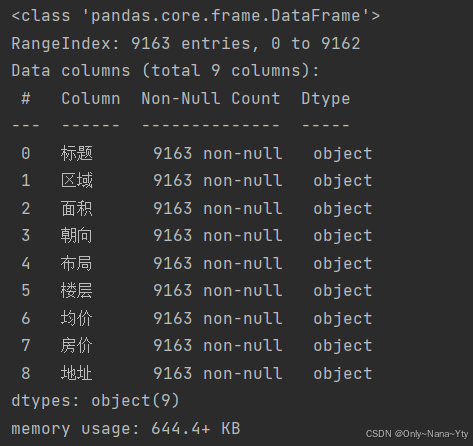
2、数据预处理
# 统计空值数量并去除
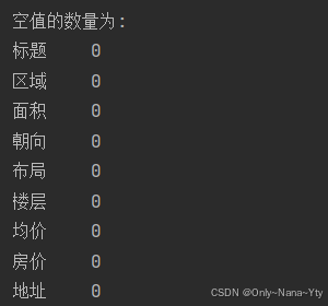
count_NaN = df.isnull().sum()
print(f'空值的数量为:\n{count_NaN}')
df = df.dropna()
# 删除重复行
df = df.drop_duplicates()
# 除去数据中不符合标准的值
df = df[df['面积'].str.contains('㎡')]
# 去除面积异常值
df =df[df['面积'].map(lambda x: float(x[:-1]))>0]
# 修改列名
df = df.rename(columns={'均价':'房价','房价':'总价'})
# 对面积进行数据提取
df['面积'] = df['面积'].map(lambda x: float(x[:-1]))
# 房价
df['房价'] = df['房价'].map(lambda x:float(x[:-3]))
# 布局
df['卧室数量'] = df['布局'].map(lambda x:int(x[:1]))
df['客餐厅数'] = df['布局'].map(lambda x:int(x[2:3]))
# 对数据列进行重新排序
columns = ['标题','区域','面积','朝向','布局','卧室数量','客餐厅数','楼层','总价','地址','房价']
df = pd.DataFrame(df,columns=columns)
为了更好地筛选出具有研究意义的数据,这里对房价和面积的数据分布进行了统计
# 房价数据分布
plt.figure(figsize=(8, 6), dpi=100)
plt.hist(df['房价'],zorder=2)
plt.xlabel('房价(元/㎡)', fontsize = 14)
plt.ylabel("频次",fontsize=14)
plt.title("房价分布",fontsize=20)
for spine in plt.gca().spines.values():
    spine.set_visible(False)
plt.gca().spines["bottom"].set_visible(True)
plt.savefig('./fig/房价分布.png')

# 面积数据分布
plt.figure(figsize=(8, 6), dpi=100)
plt.hist(df['面积'],zorder=2)
plt.xlabel('面积(㎡)', fontsize = 14)
plt.ylabel("频次",fontsize=14)
plt.title("面积分布",fontsize=20)
for spine in plt.gca().spines.values():
    spine.set_visible(False)
plt.gca().spines["bottom"].set_visible(True)
plt.savefig('./fig/面积分布.png')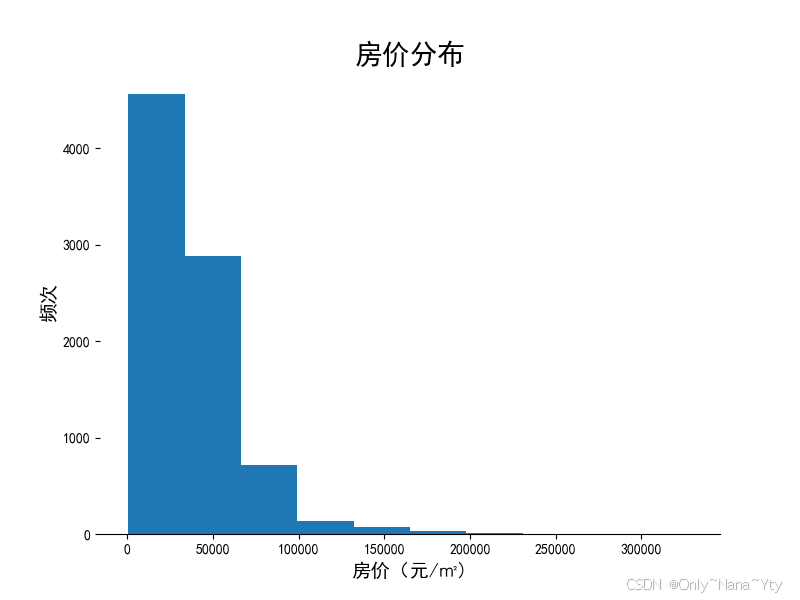
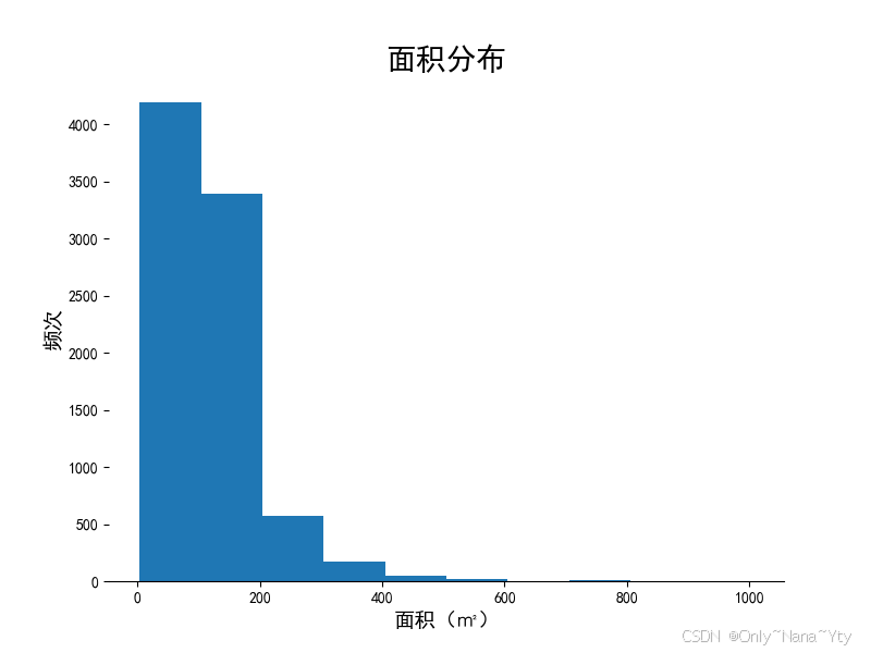
从图中可以得知房价大于200000元和面积大于500平方米的房屋数量占比极低
为排除极值对后续分析的影响,故接下来的仅统计分析房价在200000元以内且房屋面积在500平方米以内的房子
data = df.query("房价 <= 200000 & 面积 <= 500")
df.to_csv('./data/广州各区二手房数据(筛选后实验数据).csv',index=False)
二、可视化
通过可视化的形式展示各特征与房价的关系
# 获取数据
df = pd.read_csv('./data/广州各区二手房数据(筛选后实验数据).csv')
1、各区平均房价分布情况
count_region = df['区域'].value_counts()
avgprice_region = df.groupby('区域')['房价'].mean()
bars = plt.bar(avgprice_region.index, avgprice_region.values)
plt.title('广州各地区二手房数量及其平均房价分布情况', pad=20)
plt.ylabel('平均房价(元/㎡)')
# 在柱状图上添加数值显示
for bar in bars:
    height = bar.get_height()
    plt.text(bar.get_x() + bar.get_width() / 2, height + 0.2,
             f'{height:.0f}', ha='center', va='bottom', fontsize=10)

y_offset = 6000

for index, bar in enumerate(bars):  # 使用enumerate同时获取索引和bar对象
    height = bar.get_height()
    region = avgprice_region.index[index]  # 通过索引获取对应的分类标签(地区名)
    count = count_region.loc[region]  # 根据地区名获取平均房价
    plt.scatter(bar.get_x() + bar.get_width() / 2, height + y_offset, s=10, c='r', alpha=0.8, edgecolor='black',
                linewidth=1, label='房屋数量')
    # 在点旁边添加房屋数量的文本显示(可选,如果想同时显示文本便于精确查看数值)
    plt.text(bar.get_x() + bar.get_width() / 2, height + y_offset + 700,
             f'{count:.0f}', ha='center', va='bottom', fontsize=11)

plt.legend(['房屋数量'], loc='upper right')
for spine in plt.gca().spines.values():
    spine.set_visible(False)
plt.gca().spines["bottom"].set_visible(True)
# 除去y轴
# 单独隐藏y轴的刻度标签
plt.gca().set_yticklabels([])
# 隐藏y轴的刻度线
plt.gca().set_yticks([])
plt.savefig('./fig/广州各地区二手房平均房价分布情况.png')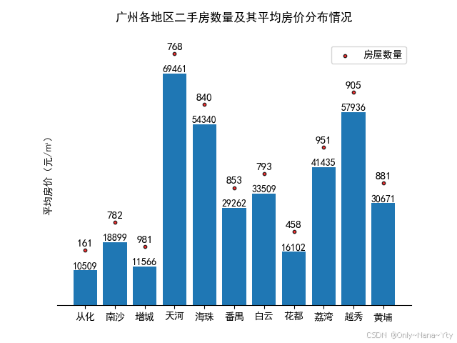
从这张图表来看,广州各地区二手房价格差异较大。
在高房价区域,天河区的平均房价最高,达到 69461 元 /㎡,这表明天河区作为广州的核心商业区,其房产价值较高。海珠区的平均房价为 54340 元 /㎡,也处于较高水平。
而在相对低房价区域,从化区的平均房价最低,为 10509 元 /㎡,其次是增城区 11566 元 /㎡和花都区 16102 元 /㎡。这些区域可能相对远离市中心,或者处于城市发展中的郊区地带。
整体来看,广州二手房价格呈现出中心区域高、外围区域低的走势。中心商务区和成熟配套区域房价较高,而城市边缘地带房价较低。
2、房价与面积的散点图
price_data = df['房价']
area_data = df['面积']
plt.scatter(price_data, area_data)
plt.title('房价与面积的散点图')
plt.xlabel('面积')
plt.ylabel('房价')
for spine in plt.gca().spines.values():
    spine.set_visible(False)
plt.gca().spines["bottom"].set_visible(True)

plt.savefig('./fig/房价与面积的散点图.png')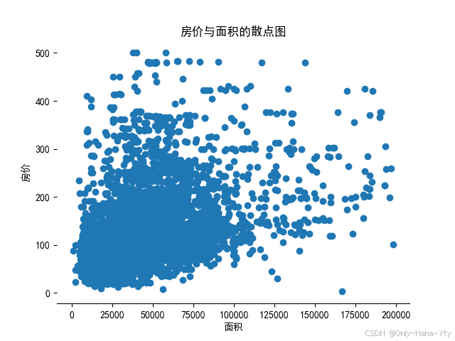
大部分数据点集中在左下角区域,表示面积较小的房屋价格也较低。随着面积的增加,房价也有上升的趋势,但数据点分布较为分散,显示出房价和面积之间并没有严格的线性关系。
3、不同朝向房屋的房价分布情况
price_direction = df.groupby('朝向')['房价'].mean()
bars = plt.bar(price_direction.index, price_direction.values)
plt.title('不同朝向房屋的房价分布情况', pad=20)
plt.ylabel('平均房价')
plt.legend(['平均房价元/㎡'])
# 在柱状图上添加数值显示
for bar in bars:
    height = bar.get_height()
    plt.text(bar.get_x() + bar.get_width() / 2, height + 0.2,
             f'{height:.0f}', ha='center', va='bottom', fontsize=10)
for spine in plt.gca().spines.values():
    spine.set_visible(False)
plt.gca().spines["bottom"].set_visible(True)
# 除去y轴
# 单独隐藏y轴的刻度标签
plt.gca().set_yticklabels([])
# 隐藏y轴的刻度线
plt.gca().set_yticks([])
plt.xticks(rotation=30)
plt.savefig('./fig/不同朝向房屋的房价分布情况.png')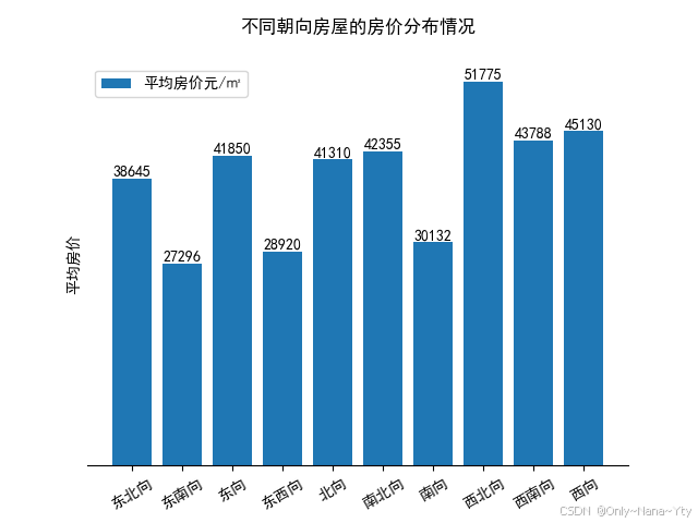
图表说明了房屋朝向对房价有显著影响,西北向的房屋最受欢迎且价格最高,而东南向的房屋价格最低。这可能与光照、通风等因素有关,西北向可能采光和视野较好,而东南向可能相对较差。
4、不同楼层房屋数量及平均房价分布情况
# 先按照楼层统计房屋数量
count_floor = df['楼层'].value_counts()

# 按照楼层分组计算平均房价
avgprice_floor = df.groupby('楼层')['房价'].mean()

# 创建一个包含两个子图的图形,共享x轴,设置图形大小
fig, (ax1, ax2) = plt.subplots(2, 1, figsize=(8, 8), sharex=True, gridspec_kw={'height_ratios': [1, 3]})

# 获取共同的楼层分类标签(确保一一对应)
common_floors = sorted(set(count_floor.index).intersection(avgprice_floor.index))

# 在第一个子图(ax1)中绘制折线图(用于展示平均房价)
# 根据共同的楼层标签来绘制折线图,确保对应关系
line = ax1.plot(common_floors, [avgprice_floor.loc[floor] for floor in common_floors], marker='o', label='平均房价')
# 在折线图的每个点上添加数值显示
for x, y in zip(common_floors, [avgprice_floor.loc[floor] for floor in common_floors]):
    ax1.text(x, y - 3000, f'{y:.0f}', ha='center', va='bottom', fontsize=10)
# 设置折线图的标题、y轴标签以及隐藏x轴相关元素(刻度、刻度标签、轴线)
ax1.set_title('不同楼层房屋数量及平均房价分布情况', pad=25)
ax1.set_ylabel('平均房价(元/㎡)')
ax1.spines['bottom'].set_visible(False)
ax1.spines['top'].set_visible(False)
ax1.spines['left'].set_visible(False)
ax1.spines['right'].set_visible(False)
# 设置y轴刻度标签为指定值
ax1.set_ylim(30000, 45000)
ax1.set_yticks([30000, 37500, 45000])
ax1.set_yticklabels(['30000', '37500', '45000'])
# # 单独隐藏x轴的刻度标签
ax1.tick_params(axis='x', which='both', bottom=False, top=False)

# 在第二个子图(ax2)中绘制柱状图(用于展示房屋数量)
# 根据共同的楼层标签来绘制柱状图,确保对应关系
bars = ax2.bar(common_floors, [count_floor.loc[floor] for floor in common_floors])
# 在柱状图上添加数值显示
for bar in bars:
    height = bar.get_height()
    ax2.text(bar.get_x() + bar.get_width() / 2, height + 0.2,
             f'{height:.0f}', ha='center', va='bottom', fontsize=10)
# 设置柱状图的标题、y轴标签以及x轴标签
ax2.set_ylabel('房屋数量')

for spine in plt.gca().spines.values():
    spine.set_visible(False)
plt.gca().spines["bottom"].set_visible(True)

# 调整子图之间的间距,使布局更合理
plt.subplots_adjust(hspace=0.2)

# 保存图片
plt.savefig('./fig/不同楼层房屋数量及平均房价分布情况.png')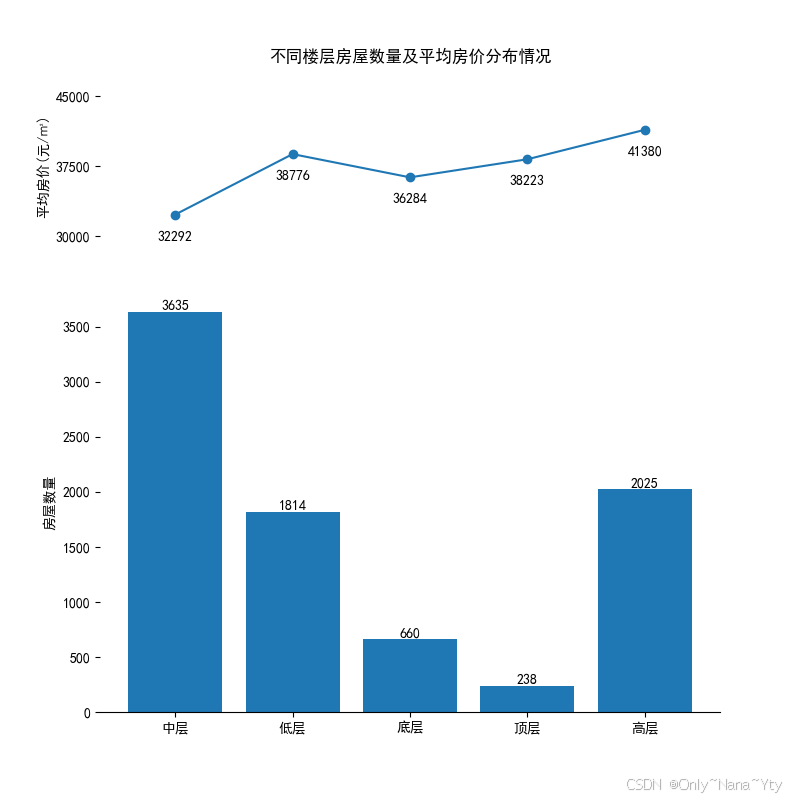
从图中可看出中层房屋数量最多,达 32292 套;高层平均房价最高,为 41380 元 /㎡。底层房屋数量最少,仅 660 套。此图显示出中层房源充足,高层价格高,底层和顶层房屋数量少。
5、房屋数量前5大布局类型占比情况
# 通过对'布局'列进行值计数来统计各布局类型的房屋数量
layout_counts = df['布局'].value_counts().reset_index()
layout_counts.columns = ['布局', '房屋数量']

# 按照房屋数量对筛选后的数据进行降序排序,并取前5名
top_5_layouts = layout_counts.sort_values(by='房屋数量', ascending=False).head(5)

# 准备数据用于绘制饼图,获取房屋数量列表
counts = top_5_layouts['房屋数量'].values

# 根据占比生成颜色列表,占比越大颜色越深
# norm = plt.Normalize(min(counts), max(counts))
# colors = plt.cm.Greens(norm(counts))
cmap = plt.get_cmap('YlOrBr_r')
colors = cmap(np.linspace(.2, .8, len(top_5_layouts)))

# 创建一个新的图形,设置图形大小
fig, ax = plt.subplots(figsize=(8, 8))

# 绘制饼图,只显示比例数值,不显示标签文字,通过设置labeldistance参数让标签不可见
explode = [0.02] * len(counts)
wedges = ax.pie(counts, startangle=90, labeldistance=1.2, colors=colors, explode=explode,
                wedgeprops={'linewidth': 1.5, 'edgecolor': 'white'})

# 绘制一个白色的圆形在中心,形成圆环图效果
centre_circle = plt.Circle((0, 0), 0.70, fc='white')
fig = plt.gcf()
fig.gca().add_artist(centre_circle)

# 在圆环内部添加比例数值
for i, wedge in enumerate(wedges[0]):
    angle = (wedge.theta1 + wedge.theta2) / 2
    x = 0.85 * np.cos(np.radians(angle))
    y = 0.85 * np.sin(np.radians(angle))
    ax.text(x, y, f'{counts[i] / sum(counts) * 100:.2f}%', ha='center', va='center', fontsize=12)

# 添加图例,将布局类型和对应的颜色展示出来
handles = [plt.Rectangle((0, 0), 1, 1, color=colors[i]) for i in range(len(top_5_layouts))]
ax.legend(handles, top_5_layouts['布局'].values, title='布局', loc='center left', bbox_to_anchor=(1, 0.5), fontsize=15)

# 设置图形标题
ax.set_title('房屋数量前5大布局类型占比情况', fontsize=17)

# 确保图形布局合理,防止标签被裁剪等情况
plt.tight_layout()

# 保存图片
plt.savefig('./fig/房屋布局类型占比情况.png')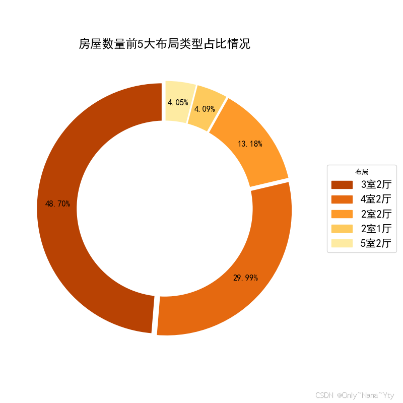
图表中可以看出前5大布局中:3 室 2 厅布局类型占比最大,为 48.70%;4 室 2 厅布局类型占比第二,为 29.99%;2 室 2 厅布局类型占比第三,为 13.18%;2 室 1 厅布局类型占比第四,为 4.09%;5 室 2 厅布局类型占比最小,为 4.05%。
6、不同卧室/客餐厅数量的平均房价变化趋势
# 获取卧室数量的平均房价
avg_price_by_bedroom = df.groupby('卧室数量')['房价'].mean().reset_index()

# 获取客餐厅数的平均房价
avg_price_by_diningroom = df.groupby('客餐厅数')['房价'].mean().reset_index()

# 创建包含两个子图的图形,共享 x 轴,设置图形大小
fig, (ax1, ax2) = plt.subplots(1, 2, figsize=(12, 6))

# 绘制卧室数量与平均房价变化趋势的折线图在第一个子图
ax1.plot(avg_price_by_bedroom['卧室数量'], avg_price_by_bedroom['房价'], marker='o')
ax1.set_title('不同卧室数量与平均房价变化趋势')
ax1.set_ylabel('平均房价')

ax1.spines['top'].set_visible(False)
ax1.spines['right'].set_visible(False)
ax1.spines['bottom'].set_visible(False)
ax1.spines['left'].set_visible(False)

# 添加水平虚线,根据y轴最大值70000合理设置步长,这里设置为每5000添加一条虚线
for y in range(25000, 65001, 5000):
    ax1.axhline(y=y, color='gray', linestyle='--', linewidth=0.5)

# 添加竖直虚线
for x in avg_price_by_bedroom['卧室数量']:
    ax1.axvline(x=x, color='gray', linestyle='--', linewidth=0.5)

# 绘制客餐厅数量与平均房价变化趋势的折线图在第二个子图
ax2.plot(avg_price_by_diningroom['客餐厅数'], avg_price_by_diningroom['房价'], marker='o')
ax2.set_title('不同客餐厅数量与平均房价变化趋势')
ax2.set_xlabel('客餐厅数量')

# 设置第二个子图 x 轴标签为整数格式
ax2.xaxis.set_major_locator(plt.MaxNLocator(integer=True))

# 添加水平虚线,根据y轴最大值70000合理设置步长,这里设置为每5000添加一条虚线
for y in range(20000, 50001, 5000):
    ax2.axhline(y=y, color='gray', linestyle='--', linewidth=0.5)

# 添加竖直虚线
for x in avg_price_by_diningroom['客餐厅数']:
    ax2.axvline(x=x, color='gray', linestyle='--', linewidth=0.5)

ax2.spines['top'].set_visible(False)
ax2.spines['right'].set_visible(False)
ax2.spines['bottom'].set_visible(False)
ax2.spines['left'].set_visible(False)

# 确保图形布局合理,防止标签被裁剪等情况
plt.tight_layout()

plt.savefig('./fig/不同卧室、客餐厅数量的平均房价变化趋势.png')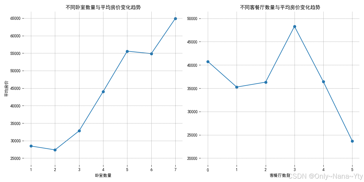
左图展示了不同卧室数量与平均房价的关系,随着卧室数量的增加,平均房价总体上呈上升趋势。2室的房屋平均房价最低,大约在 27500 元左右。7 室的房屋平均房价最高,接近 65000 元。
右图展示了不同客餐厅数量与平均房价的关系,随着客餐厅数量的增加,平均房价呈先下降后上升再下降的趋势。5客餐厅的房屋平均房价最低,在25000元以下,3客餐厅的房屋平均房价最高,在48000元左右。
7、绘制相关性热力图
df_0 = df[['区域', '面积', '朝向', '卧室数量', '客餐厅数', '楼层', '总价' ,'房价']]
## 标签化数据
from sklearn.preprocessing import LabelEncoder
lbe = LabelEncoder()
for col in df_0.columns:
    if df_0[col].dtypes == "O":
        df_0[col] = lbe.fit_transform(df_0[col])

## 绘制热力图
mask = np.array(df_0.corr())
mask[np.tril_indices_from(mask)] = False
fig, ax = plt.subplots(1, 1, figsize=(10, 10))
sns.heatmap(
    df_0.corr(),
    cmap="YlOrBr",
    annot=True,
    annot_kws={"size": 16},
    mask=mask,
    fmt='.2f',
    cbar=False,
    linewidths=2,
    linecolor="#fff"
)
ax.tick_params(labelsize=16)
plt.yticks(rotation=0)
plt.savefig('./fig/其他指标与房价的相关性热力图.png')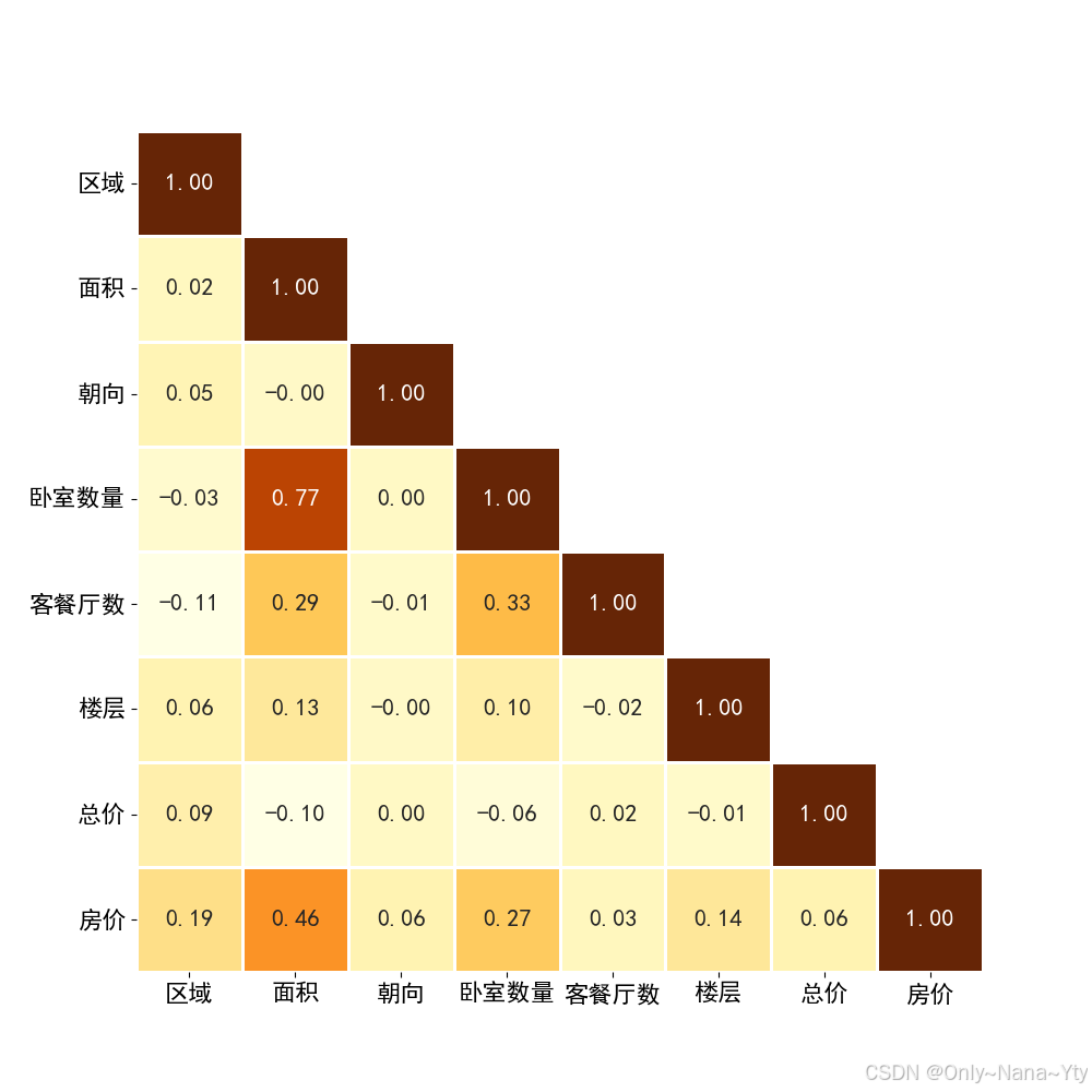
从相关性热力图中可以看出:
(i)与房价相关性最高的特征为面积,相关性值为0.46
(ii)除面积这一特征之外,其余特征均与房价呈弱正相关
三、建模预测
本节通过线性回归模型对特征进行显著性分析,再用随机森林模型对房价变化的影响因素进行预测
1、显著性分析
# 进行标签编码
label_encoder = LabelEncoder()
df['区域'] = label_encoder.fit_transform(df['区域'])
df['朝向'] = label_encoder.fit_transform(df['朝向'])
df['楼层'] = label_encoder.fit_transform(df['楼层'])
df['布局'] = label_encoder.fit_transform(df['布局'])
df['总价'] = label_encoder.fit_transform(df['总价'])
# 选择特征和目标变量
X = df.drop(columns=['标题','房价','地址'])
y = df['房价']
# 添加常数项
X = sm.add_constant(X)
# 检查X和y是否有任何非数值数据
print(X.dtypes)
print(y.dtypes)
# 建立线性回归模型
try:
model = sm.OLS(y, X).fit()
print(model.summary())
except Exception as e:
print(f"Error: {e}")
# 提取显著性分析结果
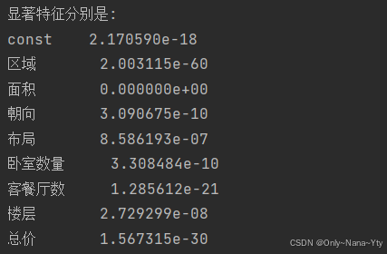
significant_features = model.pvalues[model.pvalues < 0.05]
print("Significant features:")
print(f'显著特征分别是:\n{significant_features}')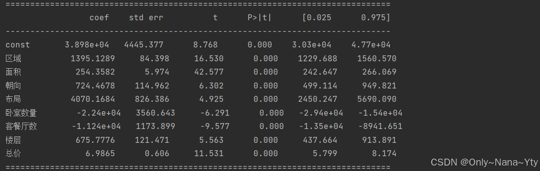
2、建模
# 提取出用于进行模型预测的特征
df_1 = df[['区域', '面积','朝向', '布局', '卧室数量', '客餐厅数', '楼层' ,'总价', '房价']]
X, y = df_1.iloc[:, :-1], df_1['房价']
X_train, X_test, y_train, y_test = train_test_split(X, y, test_size=0.2, random_state=42)
## 归一化
mms = MinMaxScaler()
X_s_train = mms.fit_transform(X_train)
X_s_test = mms.transform(X_test)
# 创建随机森林回归模型
model = RandomForestRegressor()
# 使用归一化后的训练集进行模型训练,并指定特征名称列表
model.fit(X_s_train, y_train)
y_pred = model.predict(X_s_test)
RF_score = r2_score(y_test, y_pred)
print(f"使用随机森林回归模型预测的R2得分为:{RF_score}")
# 可视化预测结果
plt.plot(y_test.values, label='true')
plt.plot(y_pred, label='pred')
plt.legend()
plt.savefig('./modelpre_fig/随机森林回归模型.png')
# 获取特征重要性
importances = model.feature_importances_
feature_names = X_train.columns.tolist()
# 绘制重要特征柱状图
plt.figure(figsize=(10, 6))
bars = plt.bar(feature_names, importances)
plt.title('随机森林特征重要性')
for bar in bars:
height = bar.get_height()
plt.text(bar.get_x() + bar.get_width() / 2, height + 0.005,
f'{height:.3f}', ha='center', va='bottom', fontsize=10)
plt.savefig('./modelpre_fig/随机森林特征重要性柱状图.png')(1)模型评估
![]()
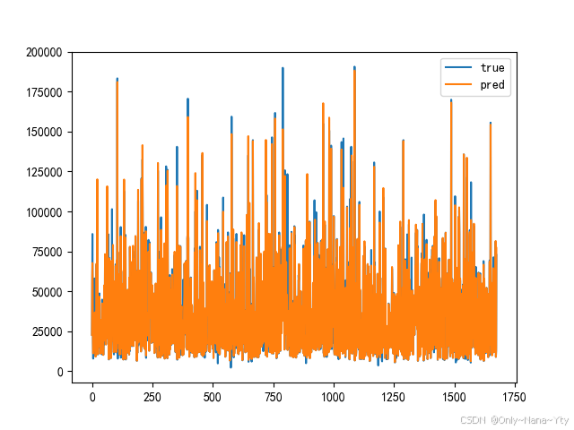
使用随机森林回归模型预测的R2得分为:0.9525013577776849,评估效果良好。根据模型预测 结果的可视化图表也可以看出随机森林模型的预测效果较好。
(2)特征重要性评价
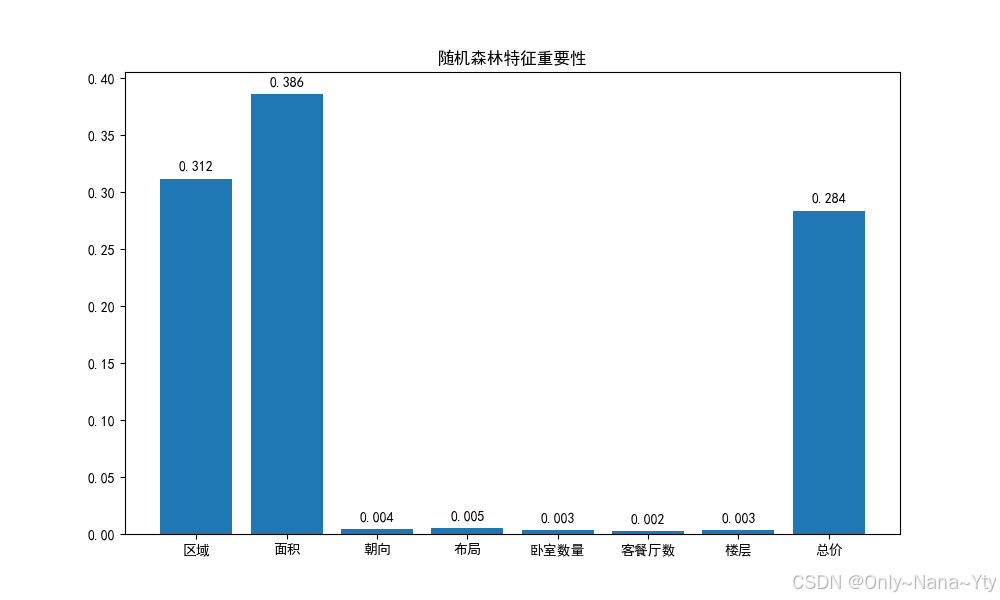
从随机森林输出的重要性特征值中可以看出:
面积是影响房价变化最重要的特征,其重要性值为 0.386。这与在通过相关性热力图进行的相关性分析中得到的结果一致。


 91
91

 被折叠的 条评论
为什么被折叠?
被折叠的 条评论
为什么被折叠?
 到【灌水乐园】发言


