Matplotlib 画动态图 animation模块的使用_matplotlib import animation(2)

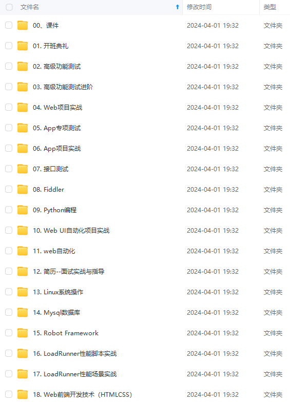
既有适合小白学习的零基础资料，也有适合3年以上经验的小伙伴深入学习提升的进阶课程，涵盖了95%以上软件测试知识点，真正体系化！

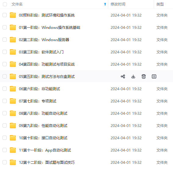
由于文件比较多，这里只是将部分目录截图出来，全套包含大厂面经、学习笔记、源码讲义、实战项目、大纲路线、讲解视频，并且后续会持续更新

需要这份系统化的资料的朋友，可以戳这里获取

xdata.append(frame)
ydata.append(np.sin(frame))
ln.set_data(xdata, ydata)
return ln,

ani = FuncAnimation(fig, update, frames=np.linspace(0, 2*np.pi, 128),
init_func=init, blit=True)
plt.show()

![sin函数动态图](https://img-blog.csdn.net/20170809165303201?watermark/2/text/aHR0cDovL2Jsb2cuY3Nkbi5uZXQvdTAxMzE4MDMzOQ==/font/5a6L5L2T/fontsize/400/fill/I0JBQkFCMA==/dissolve/70/gravity/SouthEast)


画这类图的关键是要给出不断更新的函数，这里就是*update* 函数了。注意, `line, = ax.plot([], [], 'r-', animated=False)` 中的`,` 表示创建tuple类型。迭代更新的数据`frame` 取值从`frames` 取得。


#### 例子2. 动态显示一个动点，它的轨迹是sin函数。

import numpy as np
import matplotlib.pyplot as plt
from matplotlib import animation

“”"
animation example 2
author: Kiterun
“”"

fig, ax = plt.subplots()
x = np.linspace(0, 2*np.pi, 200)
y = np.sin(x)
l = ax.plot(x, y)
dot, = ax.plot([], [], ‘ro’)

def init():
ax.set_xlim(0, 2*np.pi)
ax.set_ylim(-1, 1)
return l

def gen_dot():
for i in np.linspace(0, 2*np.pi, 200):
newdot = [i, np.sin(i)]
yield newdot

def update_dot(newd):
dot.set_data(newd[0], newd[1])
return dot,

ani = animation.FuncAnimation(fig, update_dot, frames = gen_dot, interval = 100, init_func=init)
ani.save(‘sin_dot.gif’, writer=‘imagemagick’, fps=30)

plt.show()

这里我们把生成的动态图保存为gif图片，前提要预先安装imagemagic。   
 ![sin_dot](https://img-blog.csdn.net/20170809170506942?watermark/2/text/aHR0cDovL2Jsb2cuY3Nkbi5uZXQvdTAxMzE4MDMzOQ==/font/5a6L5L2T/fontsize/400/fill/I0JBQkFCMA==/dissolve/70/gravity/SouthEast)


#### 例子3. 单摆（没阻尼&有阻尼）


无阻尼的单摆力学公式：   
 




d2θdt2+glsinθ=0

 \frac{d^2 \theta}{dt^2} + \frac{g}{l} \sin \theta = 0 
  
 附加阻尼项： 
  




d2θdt2+bmldθdt+glsinθ=0

 \frac{d^2 \theta}{dt^2} + \frac{b}{ml} \frac{d \theta}{dt} + \frac{g}{l} \sin \theta = 0 
  
 这里需要用到scipy.integrate的odeint模块，具体用法找时间再专门写一篇blog吧，动态图代码如下： 

-*- coding: utf-8 -*-

from math import sin, cos
import numpy as np
from scipy.integrate import odeint
import matplotlib.pyplot as plt
import matplotlib.animation as animation

g = 9.8
leng = 1.0
b_const = 0.2

no decay case:

def pendulum_equations1(w, t, l):
th, v = w
dth = v
dv = - g/l * sin(th)
return dth, dv

the decay exist case:

def pendulum_equations2(w, t, l, b):
th, v = w
dth = v
dv = -b/l * v - g/l * sin(th)
return dth, dv

t = np.arange(0, 20, 0.1)
track = odeint(pendulum_equations1, (1.0, 0), t, args=(leng,))
#track = odeint(pendulum_equations2, (1.0, 0), t, args=(leng, b_const))
xdata = [lengsin(track[i, 0]) for i in range(len(track))]
ydata = [-lengcos(track[i, 0]) for i in range(len(track))]

fig, ax = plt.subplots()
ax.grid()
line, = ax.plot([], [], ‘o-’, lw=2)
time_template = ‘time = %.1fs’
time_text = ax.text(0.05, 0.9, ‘’, transform=ax.transAxes)

def init():
ax.set_xlim(-2, 2)
ax.set_ylim(-2, 2)
time_text.set_text(‘’)
return line, time_text

def update(i):
newx = [0, xdata[i]]
newy = [0, ydata[i]]
line.set_data(newx, newy)
time_text.set_text(time_template %(0.1*i))
return line, time_text

ani = animation.FuncAnimation(fig, update, range(1, len(xdata)), init_func=init, interval=50)
#ani.save(‘single_pendulum_decay.gif’, writer=‘imagemagick’, fps=100)
ani.save(‘single_pendulum_nodecay.gif’, writer=‘imagemagick’, fps=100)
plt.show()

![无衰减](https://img-blog.csdn.net/20170810205911746?watermark/2/text/aHR0cDovL2Jsb2cuY3Nkbi5uZXQvdTAxMzE4MDMzOQ==/font/5a6L5L2T/fontsize/400/fill/I0JBQkFCMA==/dissolve/70/gravity/SouthEast)   
 ![衰减](https://img-blog.csdn.net/20170810210018183?watermark/2/text/aHR0cDovL2Jsb2cuY3Nkbi5uZXQvdTAxMzE4MDMzOQ==/font/5a6L5L2T/fontsize/400/fill/I0JBQkFCMA==/dissolve/70/gravity/SouthEast)


#### 例子4. 滚动的球

import numpy as np
import matplotlib.pyplot as plt
import matplotlib.animation as animation

fig = plt.figure(figsize=(6, 6))
ax = plt.gca()
ax.grid()
ln1, = ax.plot([], [], ‘-’, lw=2)
ln2, = ax.plot([], [], ‘-’, color=‘r’, lw=2)

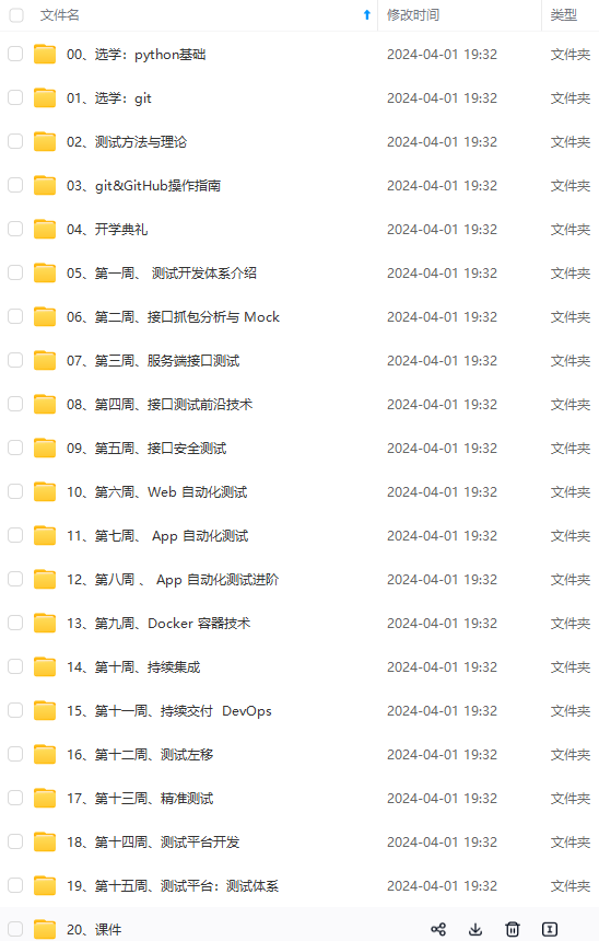
既有适合小白学习的零基础资料，也有适合3年以上经验的小伙伴深入学习提升的进阶课程，涵盖了95%以上软件测试知识点，真正体系化！

由于文件比较多，这里只是将部分目录截图出来，全套包含大厂面经、学习笔记、源码讲义、实战项目、大纲路线、讲解视频，并且后续会持续更新

需要这份系统化的资料的朋友，可以戳这里获取

的小伙伴深入学习提升的进阶课程，涵盖了95%以上软件测试知识点，真正体系化！**

由于文件比较多，这里只是将部分目录截图出来，全套包含大厂面经、学习笔记、源码讲义、实战项目、大纲路线、讲解视频，并且后续会持续更新

需要这份系统化的资料的朋友，可以戳这里获取