


基于MATLAB 水下航行器AUV/UUV 水下机器人MATLAB 六自由度基础数学模型(带参数)程序

文章目录
水下航行器(AUV/UUV)的六自由度数学模型通常包括位置和姿态的变化,这六个自由度分别是:沿X轴、Y轴、Z轴的平移运动以及绕这三个轴的旋转运动。下面提供一个简化的MATLAB代码示例,用于描述一个基础的六自由度数学模型。
六自由度数学模型
在建立六自由度模型时,我们首先需要定义航行器的位置向量 ( \mathbf{r} = [x, y, z]^T ) 和姿态角向量 ( \boldsymbol{\theta} = [\phi, \theta, \psi]^T ),其中 ( \phi ), ( \theta ), ( \psi ) 分别代表横滚角、俯仰角和偏航角。此外,还需要考虑速度向量 ( \mathbf{v} ) 和角速度向量 ( \boldsymbol{\omega} )。
动力学方程
水动力学方程可以分为两个部分:线性加速度和角加速度。
- 线性加速度:[ \dot{\mathbf{v}} = \mathbf{M}^{-1} (\mathbf{f} - \mathbf{C}(\mathbf{v})\mathbf{v} - \mathbf{D}(\mathbf{v})\mathbf{v} + \mathbf{g}) ]
- 角加速度:[ \dot{\boldsymbol{\omega}} = \mathbf{J}^{-1} (\mathbf{T} - \boldsymbol{\omega} \times \mathbf{J}\boldsymbol{\omega}) ]
其中:
- ( \mathbf{M} ) 是质量矩阵。
- ( \mathbf{f} ) 是作用力向量。
- ( \mathbf{C}(\mathbf{v}) ) 和 ( \mathbf{D}(\mathbf{v}) ) 分别是科里奥利效应和阻尼效应矩阵。
- ( \mathbf{g} ) 是重力/浮力向量。
- ( \mathbf{J} ) 是转动惯量矩阵。
- ( \mathbf{T} ) 是扭矩向量。
MATLAB 示例代码
以下是一个简化的MATLAB代码示例,用于模拟一个基本的六自由度AUV模型。
% 参数设置
m = 100; % 质量 (kg)
Ixx = 5; Iyy = 6; Izz = 7; % 转动惯量 (kg*m^2)
Xu = -50; Yv = -60; Zw = -70; % 线性阻尼系数 (N/(m/s))
Kp = -80; Mq = -90; Nr = -100; % 角速度阻尼系数 (N*m/(rad/s))

% 初始条件
x0 = [0, 0, 0]; % 初始位置 (m)
v0 = [0, 0, 0]; % 初始速度 (m/s)
theta0 = [0, 0, 0]; % 初始姿态角 (rad)
omega0 = [0, 0, 0]; % 初始角速度 (rad/s)

% 时间设置
tspan = [0 100]; % 时间范围 (s)
dt = 0.1; % 时间步长 (s)

% 定义状态变量
state0 = [x0, v0, theta0, omega0];

% ODE求解器
options = odeset('RelTol',1e-6,'AbsTol',1e-6);

[t, state] = ode45(@(t,state) dynamics(t, state, m, Ixx, Iyy, Izz, Xu, Yv, Zw, Kp, Mq, Nr), tspan, state0, options);

% 提取结果
x = state(:,1:3); % 位置
v = state(:,4:6); % 速度
theta = state(:,7:9); % 姿态角
omega = state(:,10:12); % 角速度

% 绘制结果
figure;
subplot(2,2,1);
plot(t, x); title('Position');
legend('x','y','z');

subplot(2,2,2);
plot(t, v); title('Velocity');
legend('vx','vy','vz');

subplot(2,2,3);
plot(t, theta); title('Orientation');
legend('\phi','\theta','\psi');

subplot(2,2,4);
plot(t, omega); title('Angular Velocity');
legend('\omega_x','\omega_y','\omega_z');

function dstate_dt = dynamics(~, state, m, Ixx, Iyy, Izz, Xu, Yv, Zw, Kp, Mq, Nr)
    % 解包状态变量
    x = state(1:3); % 位置
    v = state(4:6); % 速度
    theta = state(7:9); % 姿态角
    omega = state(10:12); % 角速度

    % 计算旋转矩阵 R_b_to_i
    phi = theta(1); theta_val = theta(2); psi = theta(3);
    R_b_to_i = [cos(theta_val)*cos(psi), sin(phi)*sin(theta_val)*cos(psi)-cos(phi)*sin(psi), cos(phi)*sin(theta_val)*cos(psi)+sin(phi)*sin(psi);
                cos(theta_val)*sin(psi), sin(phi)*sin(theta_val)*sin(psi)+cos(phi)*cos(psi), cos(phi)*sin(theta_val)*sin(psi)-sin(phi)*cos(psi);
                -sin(theta_val), sin(phi)*cos(theta_val), cos(phi)*cos(theta_val)];

    % 计算角速度到体坐标系的转换矩阵 T
    T = [1, sin(phi)*tan(theta_val), cos(phi)*tan(theta_val);
         0, cos(phi), -sin(phi);
         0, sin(phi)/cos(theta_val), cos(phi)/cos(theta_val)];

    % 力和扭矩
    f = [0; 0; 0]; % 外部力 (N)
    T = [0; 0; 0]; % 外部扭矩 (N*m)

    % 阻尼力和扭矩
    C_v = diag([Xu, Yv, Zw]);
    C_omega = diag([Kp, Mq, Nr]);
    D_v = C_v * v;
    D_omega = C_omega * omega;

    % 动力学方程
    dv_dt = inv(m) * (f - D_v);
    domega_dt = inv([Ixx, 0, 0; 0, Iyy, 0; 0, 0, Izz]) * (T - cross(omega, [Ixx, Iyy, Izz] .* omega));

    % 积分更新
    dx_dt = R_b_to_i * v;
    dtheta_dt = T * omega;

    % 返回导数
    dstate_dt = [dx_dt; dv_dt; dtheta_dt; domega_dt];
end
这段代码通过定义一个简单的六自由度动态模型来模拟AUV的运动,并使用ode45求解器进行数值积分。这个模型非常简化,实际应用中可能需要考虑更多因素,如非线性效应、流体动力学参数等。根据具体需求调整参数和模型结构将有助于获得更准确的结果。
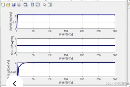
假设这是一个典型的六自由度(6-DOF)水下航行器(AUV/UUV)模型的仿真结果。
假设的信号
- 第一个信号可能是线速度 ( v_x )。
- 第二个信号可能是线速度 ( v_y )。
- 第三个信号可能是线速度 ( v_z )。
- 第四个信号可能是角速度 ( \omega_z )。
MATLAB/Simulink 代码示例
1. 定义系统参数和初始条件
% 系统参数
m = 100; % 质量 (kg)
Ixx = 5; Iyy = 6; Izz = 7; % 转动惯量 (kg*m^2)
Xu = -50; Yv = -60; Zw = -70; % 线性阻尼系数 (N/(m/s))
Kp = -80; Mq = -90; Nr = -100; % 角速度阻尼系数 (N*m/(rad/s))

% 初始条件
x0 = [0, 0, 0]; % 初始位置 (m)
v0 = [0, 0, 0]; % 初始速度 (m/s)
theta0 = [0, 0, 0]; % 初始姿态角 (rad)
omega0 = [0, 0, 0]; % 初始角速度 (rad/s)

% 时间设置
tspan = [0 300]; % 时间范围 (s)
dt = 0.1; % 时间步长 (s)

% 定义状态变量
state0 = [x0, v0, theta0, omega0];
2. 定义动力学方程
function dstate_dt = dynamics(t, state, m, Ixx, Iyy, Izz, Xu, Yv, Zw, Kp, Mq, Nr)
    % 解包状态变量
    x = state(1:3); % 位置
    v = state(4:6); % 速度
    theta = state(7:9); % 姿态角
    omega = state(10:12); % 角速度

    % 计算旋转矩阵 R_b_to_i
    phi = theta(1); theta_val = theta(2); psi = theta(3);
    R_b_to_i = [cos(theta_val)*cos(psi), sin(phi)*sin(theta_val)*cos(psi)-cos(phi)*sin(psi), cos(phi)*sin(theta_val)*cos(psi)+sin(phi)*sin(psi);
                cos(theta_val)*sin(psi), sin(phi)*sin(theta_val)*sin(psi)+cos(phi)*cos(psi), cos(phi)*sin(theta_val)*sin(psi)-sin(phi)*cos(psi);
                -sin(theta_val), sin(phi)*cos(theta_val), cos(phi)*cos(theta_val)];

    % 计算角速度到体坐标系的转换矩阵 T
    T = [1, sin(phi)*tan(theta_val), cos(phi)*tan(theta_val);
         0, cos(phi), -sin(phi);
         0, sin(phi)/cos(theta_val), cos(phi)/cos(theta_val)];

    % 力和扭矩
    f = [0; 0; 0]; % 外部力 (N)
    T = [0; 0; 0]; % 外部扭矩 (N*m)

    % 阻尼力和扭矩
    C_v = diag([Xu, Yv, Zw]);
    C_omega = diag([Kp, Mq, Nr]);
    D_v = C_v * v;
    D_omega = C_omega * omega;

    % 动力学方程
    dv_dt = inv(m) * (f - D_v);
    domega_dt = inv([Ixx, 0, 0; 0, Iyy, 0; 0, 0, Izz]) * (T - cross(omega, [Ixx, Iyy, Izz] .* omega));

    % 积分更新
    dx_dt = R_b_to_i * v;
    dtheta_dt = T * omega;

    % 返回导数
    dstate_dt = [dx_dt; dv_dt; dtheta_dt; domega_dt];
end
3. 运行仿真
% ODE求解器
options = odeset('RelTol',1e-6,'AbsTol',1e-6);

[t, state] = ode45(@(t,state) dynamics(t, state, m, Ixx, Iyy, Izz, Xu, Yv, Zw, Kp, Mq, Nr), tspan, state0, options);

% 提取结果
x = state(:,1:3); % 位置
v = state(:,4:6); % 速度
theta = state(:,7:9); % 姿态角
omega = state(:,10:12); % 角速度

% 绘制结果
figure;
subplot(2,2,1);
plot(t, v(:,1)); title('Linear Velocity in X');
legend('vx');

subplot(2,2,2);
plot(t, v(:,2)); title('Linear Velocity in Y');
legend('vy');

subplot(2,2,3);
plot(t, v(:,3)); title('Linear Velocity in Z');
legend('vz');

subplot(2,2,4);
plot(t, omega(:,3)); title('Angular Velocity in Z');
legend('\omega_z');
说明
dynamics函数:定义了六自由度的动力学方程。ode45求解器:用于数值积分,求解微分方程。plot函数:用于绘制仿真结果。
请根据您的具体需求调整参数和模型结构。如果您有更具体的模型或参数,请提供详细信息,以便进一步优化代码。
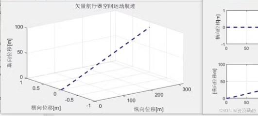
三维轨迹绘制
% 绘制三维轨迹
figure;
plot3(x(:,1), x(:,2), x(:,3), 'b.-');
xlabel('横向位移 (m)');
ylabel('纵向位移 (m)');
zlabel('垂向位移 (m)');
title('矢量航行器空间运动轨迹');
grid on;
这样,您可以得到三维空间中的运动轨迹图。希望这些代码和说明对您有所帮助!


 982
982

 被折叠的 条评论
为什么被折叠?
被折叠的 条评论
为什么被折叠?
 到【灌水乐园】发言


