Khan Academy - Statistics and Probability - Unit 4 MODELING DATA DISTRIBUTIONS

最新推荐文章于 2023-12-30 16:31:30 发布

头围五十八

最新推荐文章于 2023-12-30 16:31:30 发布

阅读量764

点赞数 3

本文链接：https://blog.csdn.net/AbCdEf_0111/article/details/107955974

版权

Khan Academy - Statistics and Proba 专栏收录该内容

7 篇文章

订阅专栏

MODELING DATA DISTRIBUTIONS

PART 1 Percentiles

PART 2 Z-scores

PART 3 Effects of linear transformation

PART 4 Density curves

PART 5 Normal distribution and the empirical rule

PART 6 Normal distribution calculations

PART 7 More on normal distributions

PART 1 Percentiles

1. Calculating percentile

(1) Method1: percent of the data that is below the amount in question

(2) Method2: percent of the data that is at or below the amount

2. Frequency, Relative frequency, Cumulative relative frequency

(1) Frequency: the number of times a given data occurs in a data set.

(2) Relative frequency: the fraction or proportion of times a given data occurs.

(3) Cumulative relative frequency: the accumulation of the previous relative frequencies.

PART 2 Z-scores

1. Z-score / Standard score: gives you an idea of how far from the mean a data point is. More technically, it measures how many standard deviations above or below the mean a data point is.

2. Formula: $z = \frac{x-\mu}{\sigma}$

3. Important facts of z-score:

(1) a positive z-score means the data point is above average

(2) a negative z-score means the data point is below average

(3) a z-score close to 0 means the data point is close to average

(4) a data point can be considered unusual is its z-score is above 3 or below -3

(5) Z-score can be applied to any distribution. It just means how many standard deviations you are away from the mean.

[NOTE] the “unusual” guideline is not an absolute rule. Some may say that a z-score beyond $\pm2$ is unusual, while beyond $\pm3$ is highly unusual. Some may use $\pm2.5$ as the cutoff.

4. Comparing the z-scores

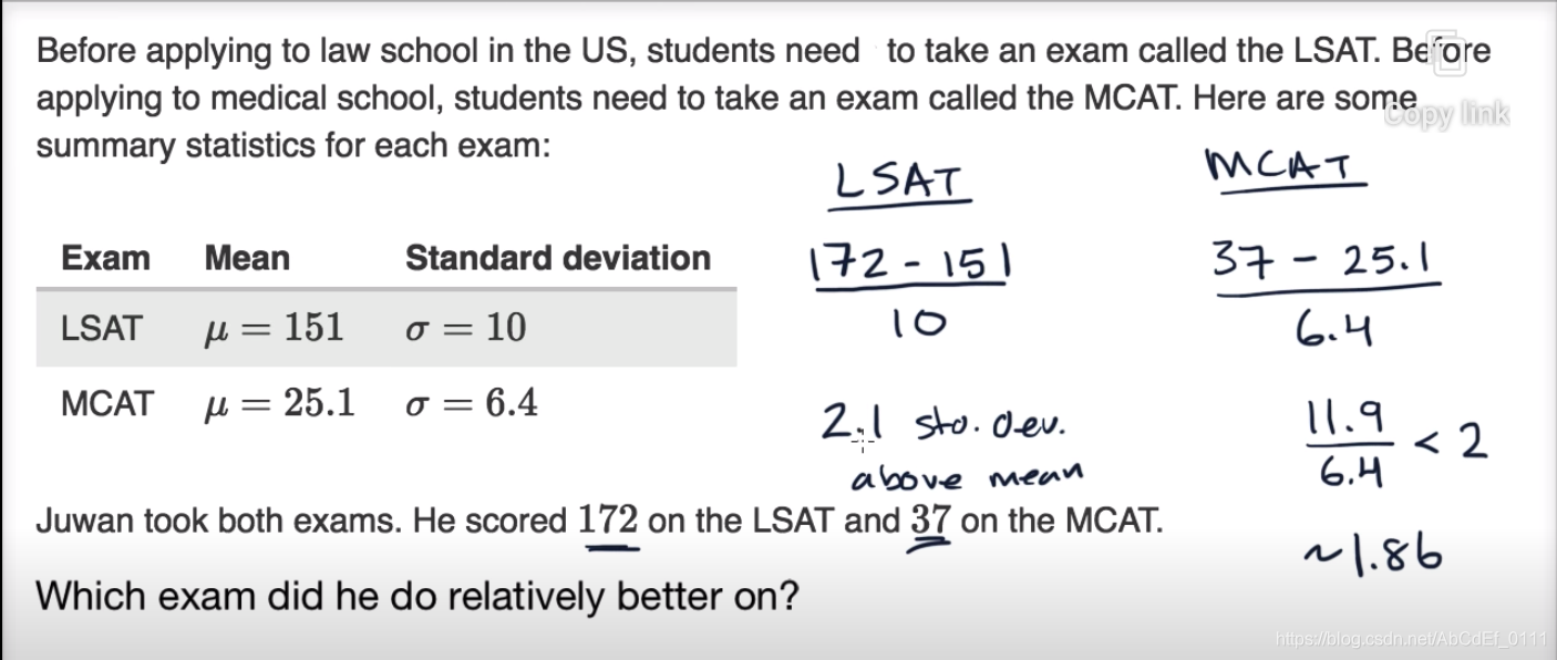
He did slightly better on the LSAT because he did more standard deviations above the mean. And because 2.1 is close to 1.86, we can say that these two scores are comparable.

5. Z-score allows us to calculate the probability of a score occurring within a normal distribution and enables us to compare two scores that are from different normal distributions.

PART 3 Effects of linear transformation

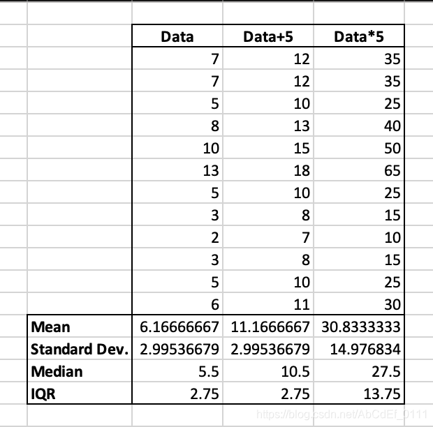
1. If the data is shifted (adding a constant to each data point in the dataset) by 1 unit:

the measures of the center will increase by 1
the measures of the spread will be affected

2. If the data is scaled (multiplying a constant to each data point in the dataset) by 10 units:

both the measures of center and spread will increase by a multiple of 10

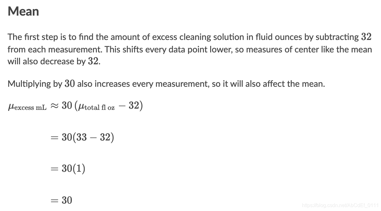
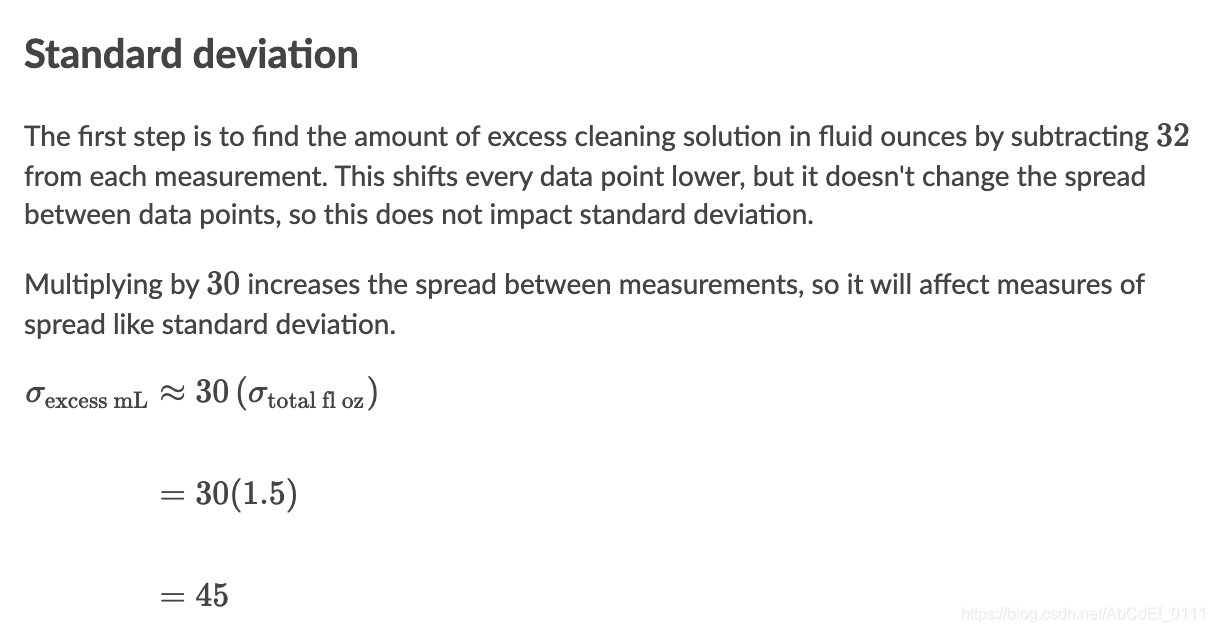
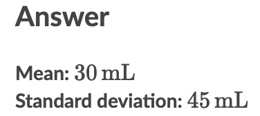
[eg]The amount of cleaning solution a company fills its bottles with has a mean of 33 fl oz and a standard deviation of 1.5fl oz. The company advertises that these bottles have 32fl oz of cleaning solution. What will be the mean and standard deviation of the distribution of excess cleaning solution, in milliliters? (1fl oz is approximately 30mL.)

PART 4 Density curves

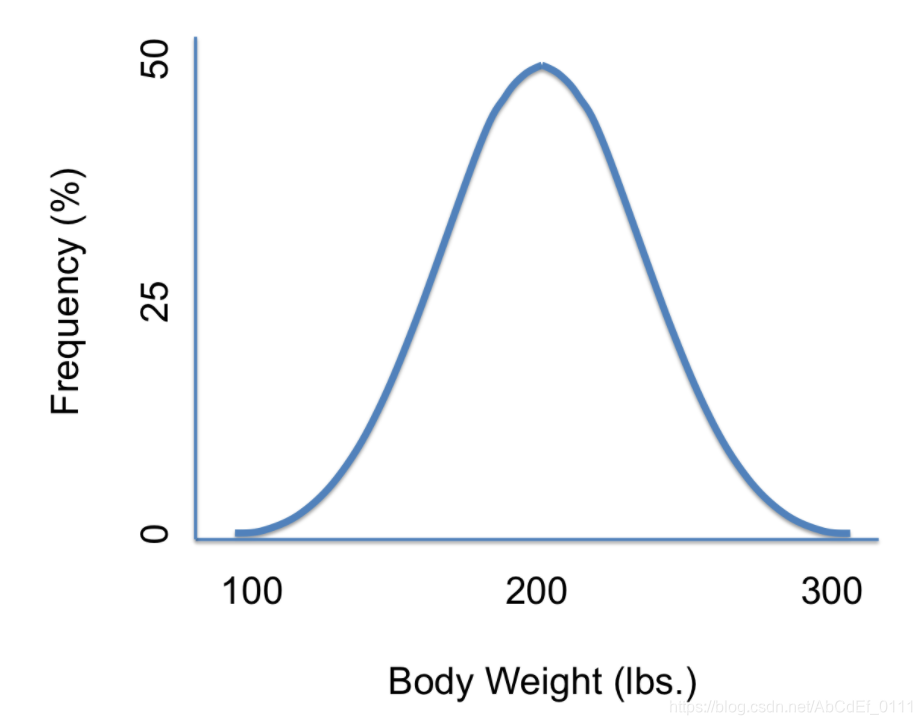
1. Density curve: is a graph that shows probability. The area under the density curve is equal to 100% OR 1

[eg] The density curve of how body weights are distributed:

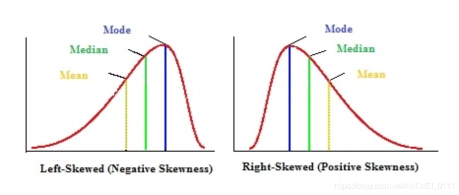
2. Mean, median, and skew from density curves

(1) Density curves can be a skewed distribution

(2) The right- or left-skew doesn’t refer to how the graph looks, it refers to whether the data is skewed

(3) A right-skewed graph will have the mean to the right to the median, and vice versa.

3. Properties of continuous probability density functions:

(1) The outcomes are measured, not counted

(2) The entire area under the curve and above the x-axis is equal to one

(3) Probability is found for intervals of $x$ values, rather than for individual $x$ values

(4) $P(c<x<d)$ is the probability that the random variable $X$ is in the interval between the values $c$ and $d$ . It is the area under the curve, above the x-axis, to the right of $c$ and the left of $d$

(5) $P(x=c) = 0$ . The probability that $x$ takes on any single individual value is zero.

(6) $P(c<x<d)$ is the same as $P(c\leqslant x\leqslant d)$ because the probability is equal to the area.

PART 5 Normal distribution and the empirical rule

1. Normal distribution: is a probability function that describes how the values of a variable are distributed.

2. Features of normal distribution:

(1) symmetric bell shape

(2) mean and median are equal; both located at the center of the distribution

(3) most of the observations cluster around the central peak

(4) extreme values in both tails of the distribution are similarly unlikely.

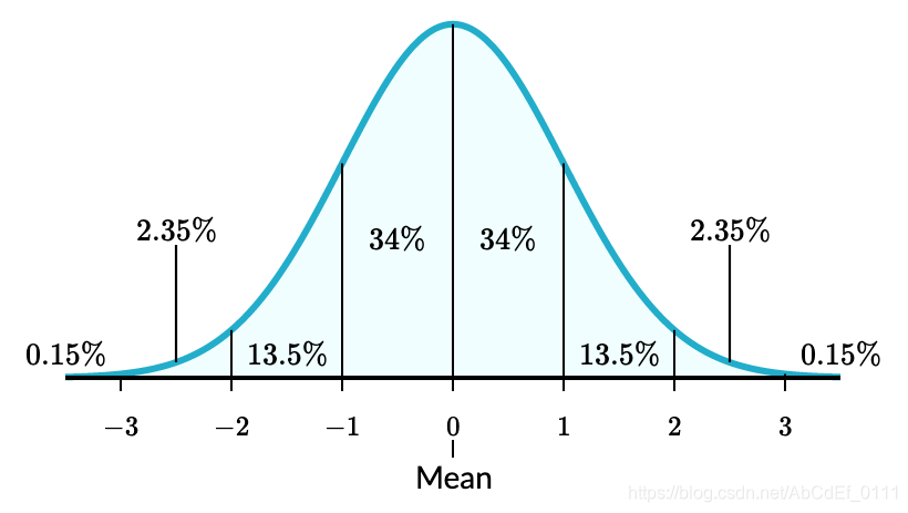
3. Empirical rule for the normal distribution

(1) around 68% of the data falls within 1 standard deviation of the mean

(2) around 95% of the data falls within 2 standard deviations of the mean

(3) around 99% of the data falls within 3 standard deviations of the mean

4. Standard normal distribution

(1) The normal distribution has many different shapes depending on the parameter values (mean and standard deviation)

(2) The standard deviation is a special case of the normal distribution where the mean is zero and the standard deviation is 1.

PART 6 Normal distribution calculations

1. Z table: A z-table, also called the standard normal table, is a mathematical table that allows us to know the percentage of values below a z-score in a standard normal distribution.

2. Standard normal table for proportion below

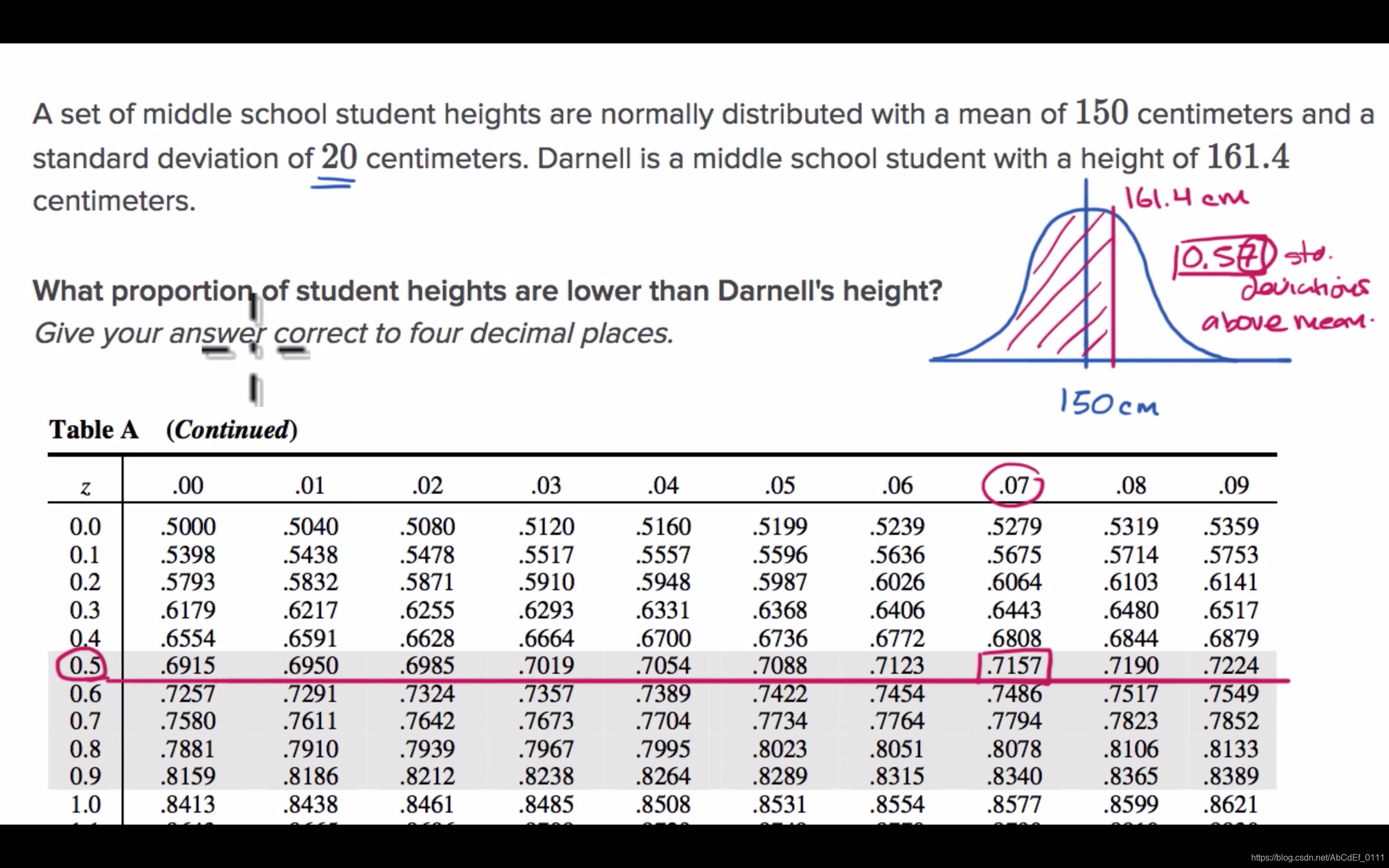
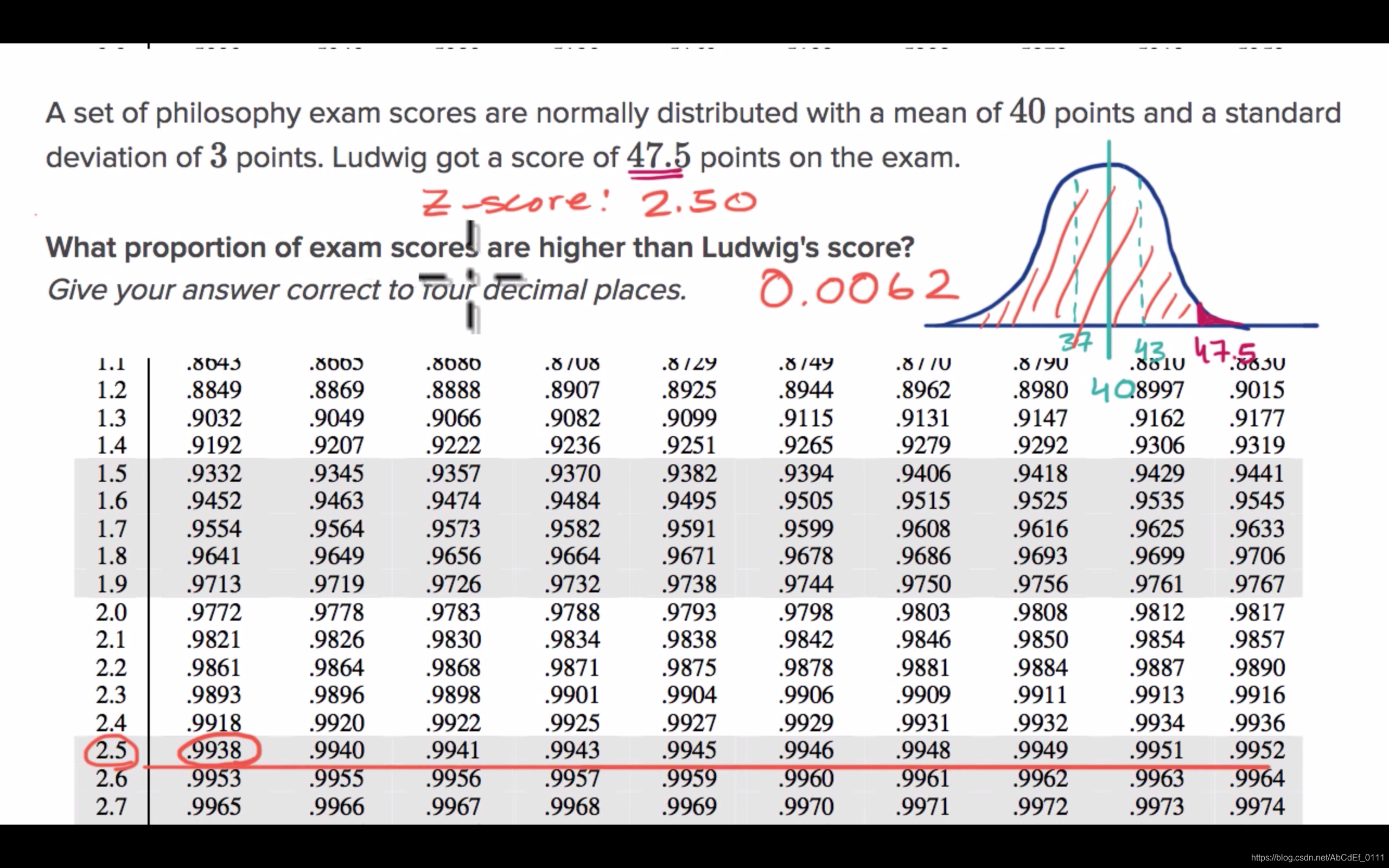
3. Standard normal table for proportion above

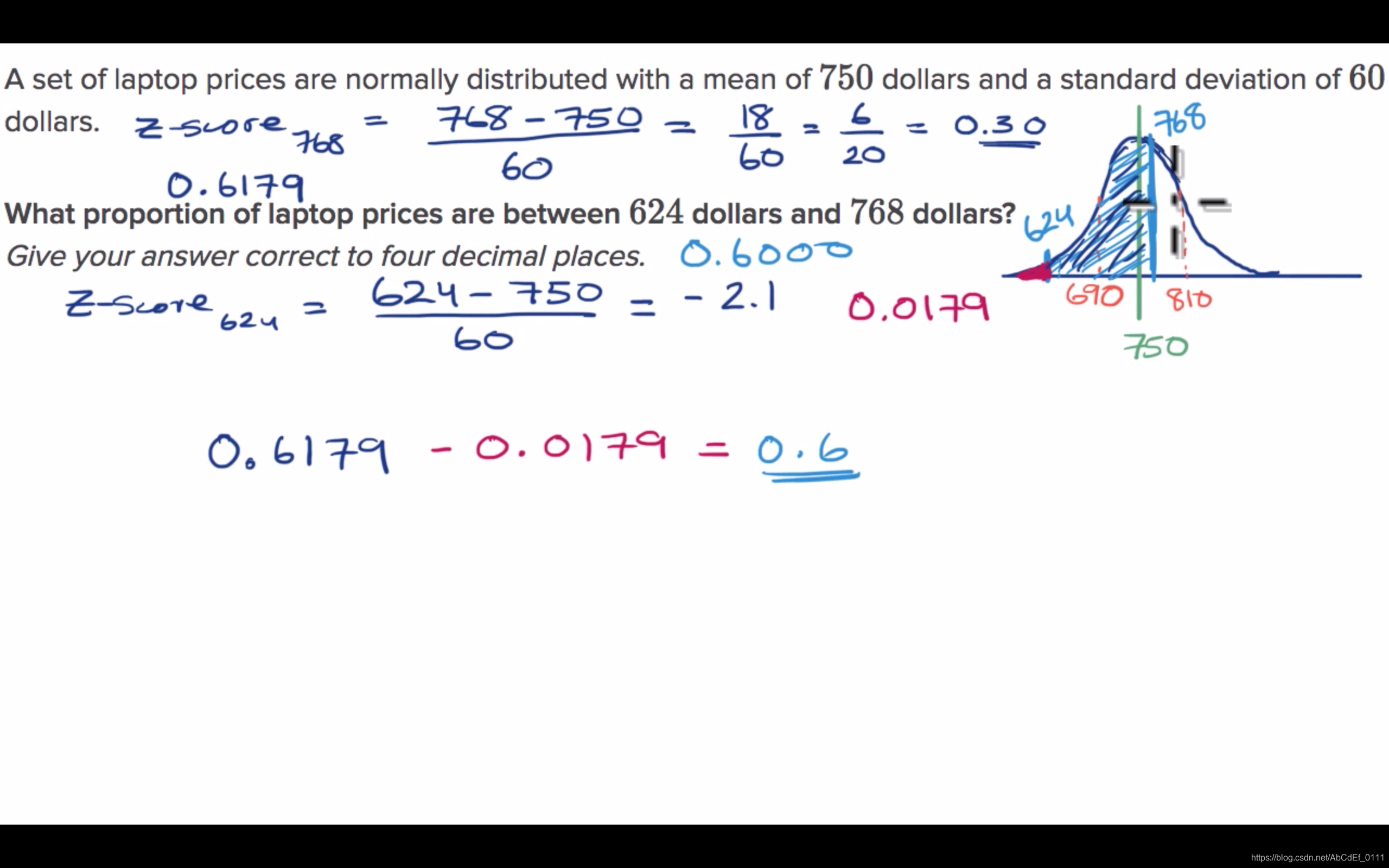
4. Standard normal table for proportion between values

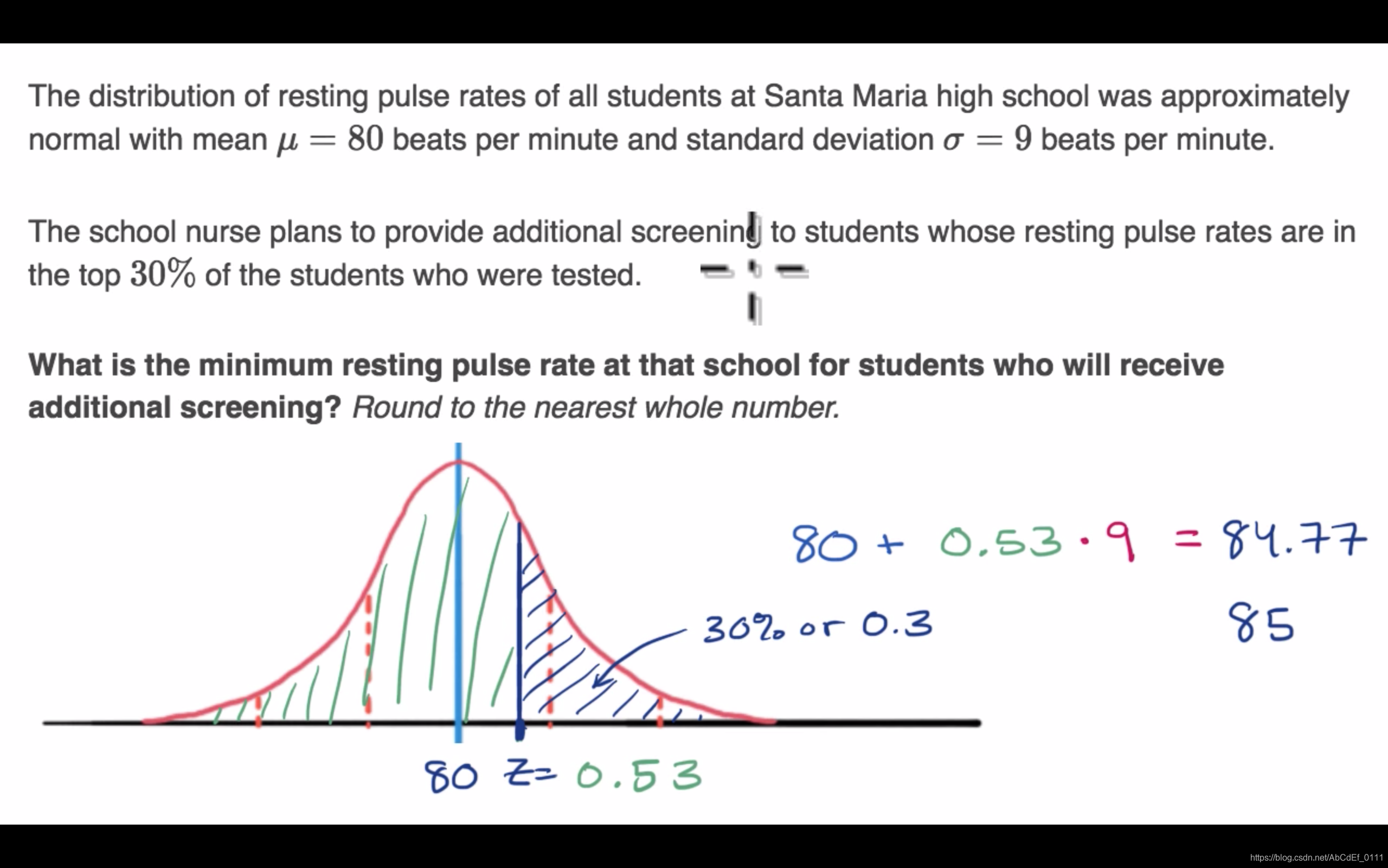
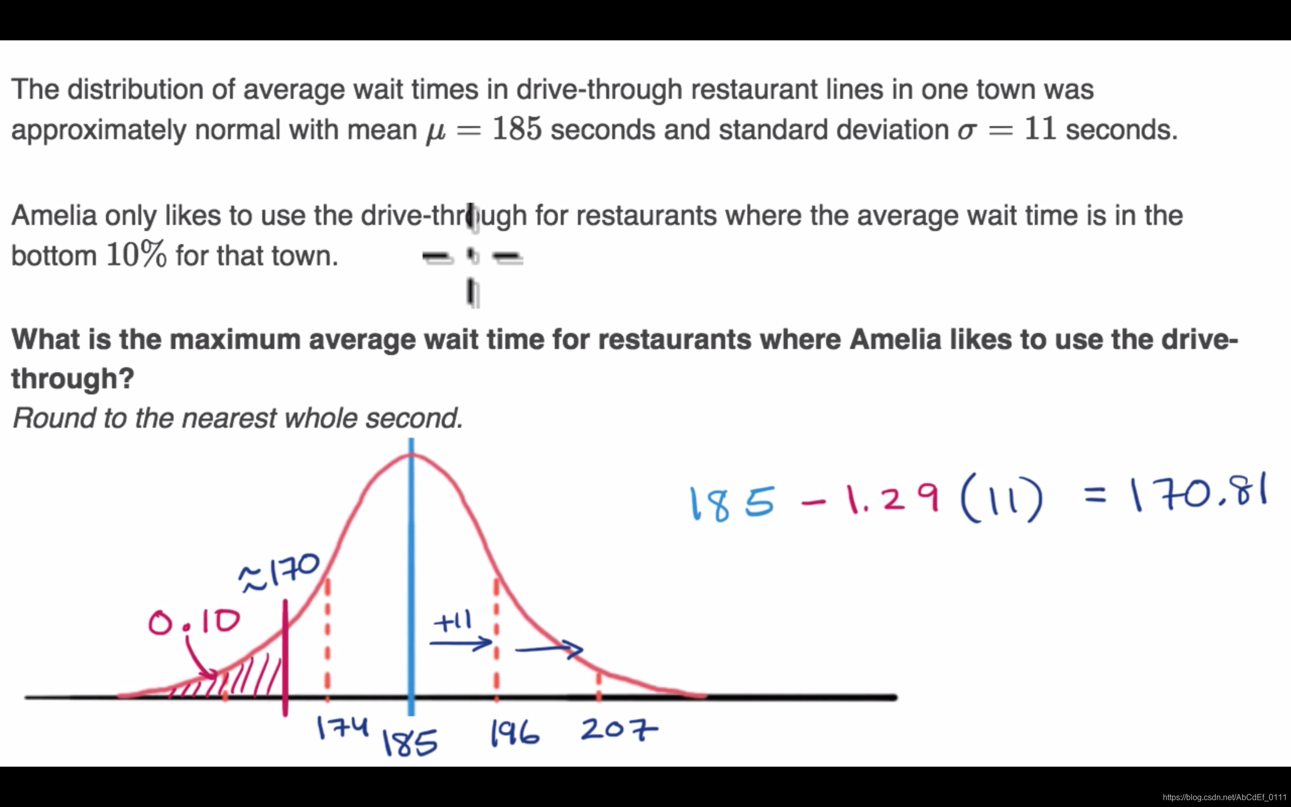
5. Finding z-score for percentile

要注意临界值:

当要找小于10%的可能性时，在z值表中要找最接近于10%，且小于等于10%对应的格子。

PART 7 More on normal distributions

1. Why normal distribution is important?

(1) Some statistical hypothesis tests assume that the data follow a normal distribution.

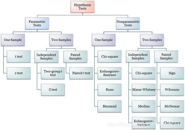
Hypothesis test hierarchy

(2) Linear and nonlinear regression both assumes that the residuals follow a normal distribution

(3) The central limit theorem states that as the sample size increases, the sampling distribution of the mean follows a normal distribution even when the underlying distribution of the original variable is non-normal.

Central limit theorem: if you have a population with mean $\mu$ and standard deviation $\sigma$ and take sufficiently large random samples from the population with replacement, then the distribution of the sample means will be approximately normally distributed.

2. Normal distribution plays an important role in inferential statistics. Inferential statistics use a random sample to draw conclusions about a population because it is not practical to obtain data from all population members.

3. Probability density function(PDF) vs. Probability mass function(PMF)

(1) PMF(概率质量函数): is a function that gives the probability that a discrete random variable is exactly equal to some value, denoted as $p(x)$ .

$p(x_i) = P(X=x_i)$

(2) PDF(概率密度函数): is the continuous analog of PMF, denoted as $f(x)$ . 连续型随机变量的概率密度函数是描述这个随机变量的输出值，在某个确定的取值点附近的可能性的函数

$P(a<X<b) = \int_{a}^{b}f(x)dx$

4. Probability density function(PDF) vs. Cumulative distribution function(CDF)

(1) CDF(分布函数): CDF of a random variable $X$ is the probability that $X$ will take a value less than or equal to $x$ , denoted as $F(x)$

$F(x) = P(X\leq x)$
$P(a<X\leq b)=F(b)-F(a)$

(2) Denote $f(x)$ as the probability density function, and $F(x)$ as the cumulative function

$\begin{aligned} f(x)&={\lim_{\Delta x \to 0}}\frac{P(x<X\leq x+\Delta x)}{\Delta x}\\ &={\lim_{\Delta x\to 0 }}\frac{F(x+\Delta x)-F(x)}{\Delta x}\\ &=F'(x) \end{aligned}$
$F(x)=P(-\infty<X\leq x) = \int_{-\infty}^{b}f(x)dx$
随机变量的X的分布函数在某一点 $x$ 的值，就是概率密度函数在 $-\infty$ 到 $x$ 上求定积分/在 $-\infty$ 到 $x$ 的线下面积

5. Normal distribution vs. Binomial distribution vs. Poisson distribution

(1) Normal distribution:

describes continuous data which have a symmetric distribution, with a characteristic ‘bell’ shape. $X$ ~ $N(\mu,\sigma^2)$
probability density function of the normal distribution: $f(x) = \frac{1}{\sigma \sqrt{2\pi}}e^{-\frac{(x-\mu)^2}{2\sigma^2}}$
In normal distribution, the probability is not coming from reading the graph, but the area under the curve.
$F(x)=P(-\infty<X\leq x) = \int_{-\infty}^{b}f(x)dx$

(2) Binomial distribution:

describes the distribution of binary data from a finite sample. Thus it gives the probability of getting $r$ events out of $n$ trials (and the probability of success in each trial is $p$ ). $X$ ~ $B(n,p)$
probability mass function of the binomial distribution: the probability of getting exactly $k$ successes in $n$ independent binomial trials is given by the probability mass function: $P(X=k) = \frac{n!}{k!(n-k)!}p^k(1-p)^{n-k}$
The normal distribution can be used as an approximation to the binomial distribution, under certain circumstances: If $X$ ~ $B(n,p)$ and if $n$ is large and/or $p$ is close to ½, then $X$ is approximately $N(np, npq)$ , where $q=1-p$

(3) Poisson distribution:

describes the distribution of binary data from an infinite sample. Thus it gives the probability of getting $r$ events in a population.
probability mass function: $P(X=k)=\frac{\lambda^ke^{-\lambda}}{k!}$