【机器学习】1.1.线性回归

包含全部示例的代码仓库见GIthub

1 导入库

import numpy as np
import matplotlib.pyplot as plt
%matplotlib inline
from sklearn.linear_model import LinearRegression

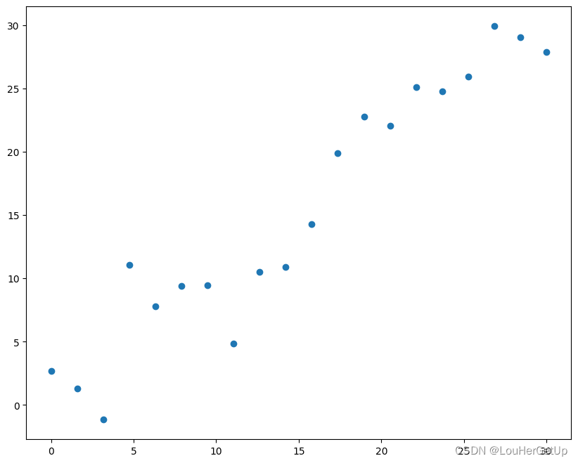
2 准备数据

x = np.linspace(0,30,20)
y = x + 3*np.random.randn(20)
x
# output
array([ 0.        ,  1.57894737,  3.15789474,  4.73684211,  6.31578947,
        7.89473684,  9.47368421, 11.05263158, 12.63157895, 14.21052632,
       15.78947368, 17.36842105, 18.94736842, 20.52631579, 22.10526316,
       23.68421053, 25.26315789, 26.84210526, 28.42105263, 30.        ])

y
# output
array([ 2.6844313 ,  1.28056793, -1.1577059 , 11.06246679,  7.81541756,
        9.38007503,  9.4664446 ,  4.82381874, 10.48489779, 10.87430035,
       14.25798235, 19.8684498 , 22.76958514, 22.06850152, 25.09763422,
       24.78744791, 25.92450483, 29.91778307, 29.04350298, 27.86164251])

plt.figure(figsize=(10,8))
plt.scatter(x,y)

3 模型构建

model = LinearRegression()

输入变成一个个的向量

X = x.reshape(-1, 1)  # 变成一个个的向量
X
# output
array([[ 0.        ],
       [ 1.57894737],
       [ 3.15789474],
       [ 4.73684211],
       [ 6.31578947],
       [ 7.89473684],
       [ 9.47368421],
       [11.05263158],
       [12.63157895],
       [14.21052632],
       [15.78947368],
       [17.36842105],
       [18.94736842],
       [20.52631579],
       [22.10526316],
       [23.68421053],
       [25.26315789],
       [26.84210526],
       [28.42105263],
       [30.        ]])

Y = y.reshape(-1, 1)

model.fit(X,Y)
model.predict([[40]])
# output
array([[40.97872639]])

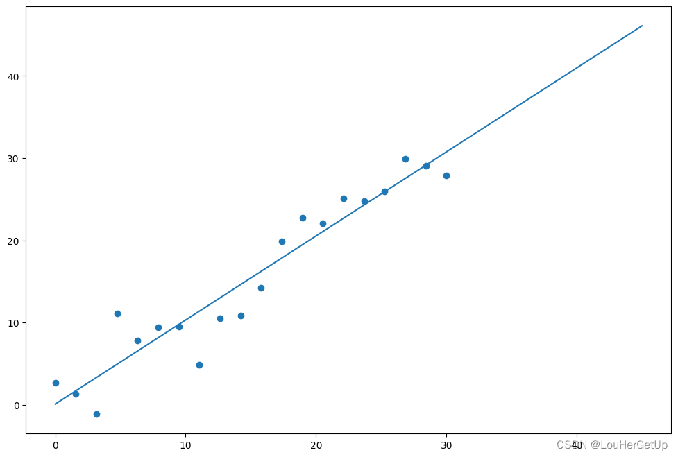
绘图

plt.figure(figsize=(12,8))
plt.scatter(x,y)
x1 = np.linspace(0,45).reshape(-1,1)
plt.plot(x1, model.predict(x1))

计算误差

Y_PRE = model.predict(X)
np.sum(np.square(Y_PRE - Y))
# output
171.24147754851296

model.intercept_  # 截距
# output
array([0.07770405])

model.coef_  # 斜率
# output
array([[1.02252556]])

调整一下预测函数，看误差是否变大

Y_PRE2 = (model.coef_ + 0.1)*X+ model.intercept_
np.sum(np.square(Y_PRE2 - Y))
# output
232.82042491693403

4 客观的评价模型

train和test的数据分布不均匀，导致模型测试结果不好

X_train, X_test = X[:10], X[10:]
Y_train, Y_test = Y[:10], Y[10:]
model = LinearRegression()
model.fit(X_train,Y_train)
np.sum(np.square(model.predict(X_test)-Y_test))
# output
609.1213719722114

调整预测函数

Y_PRE3 = model.coef_*X_test + model.intercept_ + 0.1
np.sum(np.square(Y_PRE3-Y_test))  # test 的点都在上面，数据集较小
# output
594.2234951674719

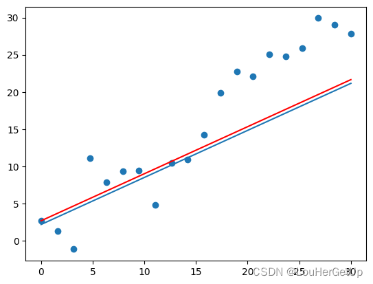
绘图，可以看出训练集和测试集分布不均匀

plt.scatter(X,Y)
plt.plot(X, model.predict(X))
plt.plot(X, model.coef_*X + model.intercept_ + 0.5, color='r')