【文献阅读】Forecasting multivariate realized stock market volatility

1、Introduction

The variances and covariances of stock returns vary over time (e.g. Andersen et al., 2005). As a result, many important financial applications require a model of the conditional covariance matrix. Three distinct categories of methods for estimating a latent conditional covariance matrix have evolved in the literature.

三种方法用于估计潜在条件方差矩阵

In the first category are the various forms of the multivariate GARCH model where forecasts of future volatility depend on past volatility and shocks (e.g. Bauwens et al., 2006).

In the second category, authors have modeled asset return variances and covariances as functions of a number of predetermined variables (e.g. Ferson, 1995).

The third category includes multivariate stochastic volatility models (e.g. Asai et al., 2006).

In this paper, we introduce a new model of the realized covariance matrix. 

We use high-frequency data to construct estimates of the daily realized variances and covariances of five size-sorted stock portfolios.

使用高频数据构建日度已实现波动率的拟合值、根据市值分类的五种资产组合的协方差

By using high-frequency data we obtain an estimate of the matrix of ‘quadratic variations and covariations’ that differs from the true conditional covariance matrix by mean zero errors (e.g. Andersen et al. (2003) and Barndorff-Nielsen and Shephard (2004a)).

通过使用高频数据，我们获得二次方差和协方差矩阵，与真实条件性协方差矩阵不同，

This provides greater power in determining the effects of alternative forecasting variables on equity market volatility when compared to efforts based on latent volatility models.

We transform the realized covariance matrix using the matrix logarithm function to yield a series of transformed volatilities which we term the log-space volatilities.

使用矩阵对数函数将已实现协方差矩阵转化为log-space volatilities.

The matrix logarithm is a non-linear function of all of the elements of the covariance matrix and thus the log-space volatilities do not correspond one- to-one with their counterparts in the realized covariance matrix.

Matrix logarithm是一种非线性函数，因此转化后log-space volatilities与已实现协方差矩阵并不一一对应。

However, modeling the time variation of the log-space volatilities is straightforward and avoids the problems that plague existing estimators of the latent volatility matrix. In particular, we do not have to impose any constraints on our estimates of the log-space volatilities.

但可以避免一些潜波动矩阵存在的问题：无用施加任何constraints。

We then model the dynamics of the log-space volatility matrix using a latent factor model. The factors consist of both past volatilities and other variables that can help forecast future volatility. We thus are able to model the conditional covariance matrix by combining a large number of forecasting variables into a relatively small number of factors.

我们使用一个潜因子模型对log-space volatiliyt的动态建模：因子包括过去波动率及其他预测变量。将大批预测变量转化为少数因子。

Indeed we show that two factors can capture the volatility dynamics of the size-sorted stock portfolios.

我们发现两个因子即可捕捉size-sorted porfolios的波动动态。

The factor model is estimated  by  GMM  yielding  a  series of filtered estimates. We then transform these fitted values, using the matrix exponential function, back  into  forecasts  of the realized covariance matrix.

拟合后，再将拟合值转化回原本形式。

Our estimated matrix is positive definite by construction and does not require any parameter restrictions to be imposed. The approach can thus be viewed as a multivariate version of standard stochastic volatility models, where the variance is an exponential function of the factors and the associated parameters.

In addition to introducing our new realized covariance matrix we also test the forecasting ability of alternative variables for time-varying equity market covariances. Our motivation is that researchers have examined a number of variables for forecasting returns but there is much less evidence that the variables forecast risks.

存在大量的预测收益研究，但预测风险相关研究较少。

The cross-section of small- and large-firm volatility has been examined in a number of earlier papers (e.g., Kroner and Ng (1998), Chan et al. (1999), and Moskowitz (2003)).

市值对波动率的影响已经被多次检验。

However, these papers used models of latent volatility to capture the variation in the covariances. In contrast, we construct daily measures of the realized covariance matrix of small and large firms over the 1988 to 2002 period. Our precise measures of volatility allow a more detailed examination of the drivers of conditional covariances than prior work.

但是，先前的研究主要是使用latent volatiliry建模。我们则用日度高频数据，更加detailed.

Naturally all of these advantages come at a cost. The main cost is that by performing our analysis on the log-space volatilities and then using the (non-linear) matrix exponential function, the estimated volatilities are not unbiased. However, as we show below, a simple bias correction is available that greatly reduces the problem.

我们的方法带来biased问题，但通过simple bias correction可以解决。

Another cost is that direct interpretation of the effects of an instrument on expected volatility is difficult due to the non-linear nature of the model.

工具变量对于预期波动的难以measure，因为其非线性的特性。

However, using our factor model estimates, we can obtain the derivatives of the realized covariance matrix with respect to the forecasting variables. We are able to calculate the derivatives at each point in our sample, yielding a series of conditional volatility elasticities that are functions of both the level of the volatility and the factors driving the volatility. The time series allows us to determine which variables have a large impact on time-varying expected volatility.

The paper is organized as follows. In Section 2, we present our model of matrix logarithmic realized volatility. In Section 3, we outline our method for constructing the realized volatility matrices and give the sources of the data. In Section 4, we give our results. In Section 5, we conclude.

2、Model

2.1 The matrix log transformation

In this paper, we use the matrix exponential and matrix logarithm functions to model the time-varying covariance matrix. The matrix exponential function performs a power series expansion on a square matrix A

 The matrix logarithm and matrix exponential functions are used in our three-step procedure to obtain forecasts of the conditional covariance matrix of stock returns. In the first step, for each day t, we use high-frequency data to construct the P  × P  realized conditional covariance matrix Vt .

第一步：对于特定t日，使用高频数据构建 P  × P 已实现条件协方差矩阵。应用矩阵对数函数，得真实对称矩阵A。

The Vt  matrix 
is positive semi-definite by construction. Applying the matrix logarithm function,

 第二步：对A矩阵的dynamics建模，整理出矩阵A对角线及以下元素获得向量a。

第三步： 使用向量a形成对称矩阵A，再应用矩阵指数函数，得到条件协方差矩阵拟合值，半正定矩阵V。

 

2.2 Factor models of volatility

2.2.1 Forecasting variables

We will use several different groups of variables to forecast the conditional covariance matrix. Based on the existing literature, we can separate the variables into two groups. The first are matrix- log values of realized volatility which are used to capture the autoregressive nature of the volatility.

使用已实现波动率的矩阵对数值，用于捕捉波动率的autoregressive nature.

There are three potential problems in using these variables to forecast volatility. First, the existing literature shows that capturing volatility dynamics will likely require a long lag structure.

To overcome this, we adapt the Heterogeneous Autoregressive model of realized volatility (HAR-RV) of Corsi (2009) and Andersen  et al. (2007) to a multivariate setting. These authors show that the aggregate market realized volatility is forecast well by a (linear) combination of lagged daily, weekly and monthly realized volatility.

 使用HAR-RV，解决RV的log lag structure。即通过多项滞后日度、周度、月度波动率的线性组合预测综合市场RV。

The second problem is that other authors have indicated that lagged realized volatility may not be the best predictor. In particular, both Andersen et al. (2007) and Ghysels et al. (2006) find that bi-power covariation – an estimate of the continuous part of the volatility diffusion – is a good predictor of the aggregate market’s realized volatility. We thus construct bi- power covariation matrices aggregated over the  and 20 days.

 and monthly log-space bi-power covariation series. In turn, these principal components are sufficient to model the realized covariance matrix.

对bi-power covariation matrix提取主成分

Our approach can thus be viewed as a multivariate approach to the HAR-RV model using the principal components of bi-power variation as predictors.

因此，我们的方法可以被视为HAR-RV模型的多元方法，使用bi-power variation的主成分作为预测因子。

The second group of forecasting variables, denoted Xt , are those variables that have been shown to forecast equity market returns.

第二类预测变量：已经证明能够预测市场收益的变量。

In equilibrium, expected returns should be related to risk, so it is natural to question whether these variables also forecast the components of market wide volatility. Below, we use a number of variables that has been shown to predict equity market returns.

We combine the two groups of forecasting variables as

Below, we select different subsets of Zt that correspond to existing approaches to modeling volatility.

2.2.2 Latent factors

结合所有预测变量建模：at为log-space波动率，Z为预测变量。a的common variation可能可以由少数因子决定。

 为了对rv matrix的common variation建模，我们使用潜因子方法。我们假设预测变量Z与潜因子存在映射关系，第K个波动率因子uk,t为Zt中N个预测变量的线性组合。

Theta为映射向量。每一个log-space波动率a为K个潜因子的函数。

 p*K个矩阵beta：log-space波动率对时变潜因子的载荷。

We note that using latent factors to model covariance matrices has a number of advantages over existing methods. First, it allows us to combine both lagged volatility measures (the principal components in (4)) as well as the Xt  variables in a  parsimonious manner. Previous models required each variable to be a separatefactor. While the large number of variables may help forecast the covariance matrix, it is unlikely that each variable represents a specific volatility factor. Our approach can be used to weigh (via the θ coefficients) all of the variables in a way that is optimal for forecasting the covariance matrix. A second advantage to our approach is that it avoids using expected returns in modeling the volatility matrix. Aggregating squared return or bi-power covariation data over high frequencies means that the expected return variation can be ignored. As the realized covariance matrix can be estimated more precisely than can the expected returns, we should obtain more precise measures of the determinants of the covariance matrix. 

 使用潜因子模型的几大好处。

2.3 Estimation

Our multivariate factor model is derived from the latent factor models of expected return variation that originated with Hansen and Hodrick (1980) and Gibbons and Ferson (1985).

我们多元潜因子模型起源

As in these papers, we estimate our factor model of volatility in (7) by GMM with the Newey and West (1987) form of the optimal weighting matrix.

使用GMM方法估计因子模型

最大步数为25的GMM迭代方法，工具变量为预测变量Z。

在公式7中，因为beta与theta结合无法求解。因此施加restrictions，即可以使用GMM求解。

Our model has a potential errors-in-variables problem as the log-space bi-power covariation matrix  is constructed with error. Using its principal components as regressors will result in biased estimates of the coefficients.

 我们的模型存在潜在的变量误差，因为 the log-space bi-power covariation matrix  （公式4）是带着误差构建的。使用其PCA将会造成有偏参数。

 GJ提出：使用工具变量回归所得beta的滞后项可以克服该偏差。我们使用该方法，并使用GMM工具集中的主成分的twice lagged values.

一旦参数被GMM估计算后，其拟合值将被分配为square matrix At. 应用矩阵指数函数得到协方差矩阵的预测值。随后，我们应用标准的预测评价计算对比两者。

2.4 Bias correction

 由于拟合在log-volatility space完成，因此我们所拟合Vt是有偏的。若A与episilon正态分布，可以使用analytic bias correction。但是我们的数据不满足该条件，因此进行简单的numerical bias correction。

其中SDt为标准差的主对角矩阵，C为相关性的对称矩阵。估计Vt类似方法分解。

我们估算偏差纠正后的因子，通过两个标准差序列的中位数。

保留相关性完整同时完成标准差的纠正。该简单的方法效果很好 。我们也承认有其他更加复杂的纠正方法可以产生更好的结果。

2.5 interpreting expected volatility

The matrix logarithmic volatility model has the disadvantage that the estimated coefficients cannot be interpreted directly as the effect of the variable on the specified element of the realized volatility.

矩阵对数波动率模型存在缺点：拟合参数无法被直接解释，即变量对rv的效应无法明确。

V和A非线性的关系导致该情况。但是，拟合矩阵V的导数与因子模型的元素的对应关系可以轻松获得。

 设A为公式3中P*P的预期条件协方差矩阵，且其为特定预测变量的矩阵。

 A(z)对z求导，即实际波动率A的导数矩阵与z是一一对应的；

因此dV(z)/dz即为公式10所示矩阵的右上板块。

通过公式10可以分析预测变量对已实现协方差矩阵的解释能力。

 我们可以计算整体样本的平均影响，或是某一点时间上的条件性影响。比如，A(zt）为dayt的realized log-space volatilities. 为了探求预期协方差矩阵对预测变量的response，我们需要计算导数。因为我们的双因子模型如公式7,可以计算，再将其代入公式10计算得时变弹性。

该弹性即为Vt第i,j的元素变化百分比，由于预测变量的一个标准差变化。因此我们可以检验资本市场方差或协方差的变化，对应于预测变量的变化。在接下来的分析中，我们将会展示弹性存在的时变效应。

3、Data

3.1 Realized volatility

We construct our realized covariance matrices from two data sets: the Institute for the Study of Securities Markets’ (ISSM) database and the Trades and Quotes (TAQ) database. Both data sets contain continuously-recorded information on stock quotes and trades for securities listed on the New York Stock Exchange (NYSE). The ISSM database provides quotes from January 1988 through December 1992 while the TAQ database provides quotes from January 1993 through December 2002.

Value-weighted portfolio returns are created by assigning stocks to one of five size-sorted portfolios based on the prior month’s ending price and shares outstanding.

计算上一个月末的价格与流通股数得市值，并将股票根据市值五等分。

Our choice of portfolios is partially motivated by an interest to see if the systematic components of conditional volatility are common across the size portfolios. We use the CRSP database to obtain shares outstanding and prior month ending prices.

条件波动的系统性成分是否会在不同市值的资产组合具有相同部分。

Once we have our time series of high-frequency portfolio returns, we construct our measure of realized covariance matrices using the approach of Hansen and Lunde (2006), who recommend a Newey and West (1987) type extension to the usual realized volatility construction.They note the potential bias in calculating variances if the serially autocorrelated nature of the data is ignored.

通过HL的方法计算已实现协方差矩阵。

Our data likely suffers from this problem as the portfolios of smaller stocks will include securities that are more illiquid than stocks in the larger quintiles. The illiquidity of small stocks suggests that price and volatility responses to information shocks may take more time to be incorporated, leading to time series autocorrelation in the high-frequency returns.

高频收益存在自相关性导致误差。

 表1描述性统计。偏度接近于0，峰度接近于3。进行矩阵对数处理的rv(at)更加接近于正态分布。

3.2 Forecasting variables

我们的目标：对比不同的条件协方差矩阵的模型。尽管所有的模型都是用公式7的潜因子模型，但所用预测变量Z不同。我们构建四种模型。

 第一种模型：MHAR-RV-BP。

使用bi-power covariation作为预测因子。多个主成分存在共线性，因此只用5天，20天的第一主成分作为预测因子。通过5天的测度希望capture高频波动率方差。

 第二种模型：MHAR-RV-BPA。

 增加了波动率对过去收益变动的非对称respones作为预测因子。

第三种模型：MHAR-RV-X。债券利率、股息率、信用价差、期限结构斜率。行为金融指标。

第四种模型：MHAR-RV-BPAX。使用所有变量。

 4、Result

4.1 Model fit

K=1被拒绝

 K=2，参数恰好不会onerous，因此后续分析使用两因子模型。

 over-identifying restrictions会导致样本内拟合的下降：

 因此在表1panelB进行检验，分子为由log-space volatilities拟合所得At的方差，即公式7所得；分子为由log-space volatilities最小二乘法拟合值方差，即公式5所示。

 该比例表示了公式8所施加的因子结构，降低了多少样本内预测能力。

In Panel C of Table 2, we measure the restrictions of the factor model on the realized volatility matrix, Vt .

Panel B测度了公式8对log-space volatility A的影响，Panel C则测度了公式8对realized volatility V的影响。

In addition, the calculations for these ratios vary by whether they are for diagonal or off-diagonal elements of Vt . For the diagonal elements, the numerator is the variance of the (bias-corrected) fitted values of the realized volatility from (9).

分子为公式9所得realized volatility:

 The denominator is the variance of the fitted values from an ordinary least squares regression of the realized volatilities on the variables of the model.

分母为最小二乘法所得方差

For the off- diagonal elements, we repeat the same exercise using the Fisher transforms of the estimated correlations in the numerator and the Fisher transforms of the realized correlations in the dominator.

对于非对角线元素，我们重复相同的过程，对分子的拟合相关性使用Fisher转换，对分母已实现相关性进行Fisher转换。

This analysis allows us to measure the effects of the factor model on both the volatilities and the correlations contained in Vt .

这使得我们可以测度：因子模型对 波动率以及Vt所包含的相关性 的影响。

尽管Panel B中矩阵A（1，4）元素的一些比率很少，但大部分都是大于0.7的，公式8的restriction似乎并没有给log-space volatilities带来太多影响；

 Panel C的结果类似，其中大于1的部分matrix exponential function允许我们捕捉更多的方差（比起简单的最小二乘法）。总而言之，表2的结果表明两因子模型并不会过于严格，预期方差的大部分方差以及相关性都被我们的模型成功capture。

 4.2 Estimated coefficients

表3呈现了beta系数的估计值，使用了所有的forecasting variables。根据矩阵A的元素一一对应得到。正交元素位于左上角。

 每一个cell表示由GMM、NW所拟合的estimation。

在第一个因子中，四个对角元素对应loadings是显著且正的，而其他的值要小很多；第二个因子类似。所有的log-space volatilities都具有至少一个因子的显著载荷。因此预测因子的线性组合能够预测矩阵A的元素。

表4A展示了MHAR-RV-BP模型的双因子系数Theta。大部分系数都是显著的。双因子系数的区别表明因子picking up different elements of long-run volatility。但是因为模型的highly non-linear nature，很难说哪个因子对realized volatility有着更多的影响。

 例如，a(20,1)的第二因子系数绝对值大于a(5,1)，并不一定说明其对realized volatility的影响就越大。

下面列出的弹性才是：the ultimate impact of any particular forecasting variable on volatilities.

Panel B presents the coefficients for the model that includes the (asymmetric) effects of past stock returns (MHAR-RV-BPA). 

4B呈现了包含过去收益非对称影响的模型系数。

 The coefficients on the lagged principal components of bi-power covariation are similar in size and significance to their values in the first model.

bi-power covariation的主成分滞后参数大小与显著性均类似于4A

In addition an interesting pattern in the asymmetric response of volatility to past negative returns emerges.

波动率对过去负向收益的非对称影响

The coefficient on lagged negative returns on small stocks is negative in the first factor and not significant in the second factor.

小市值滞后negative returns的系数：在第一个因子上为负，在第二个因子上不显著。

The coefficient on negative returns on large stocks has an opposite sign in the two factors. The elasticities presented below will show how the effects net out.

负向收益系数在两个因子上的系数相对。下述弹性将展示这些影响如何抵消。

The coefficients on the variables  usually  used  to  forecast  stock returns, model ‘MHAR-RV-X’, are presented in Panel C.

用于预测股票收益的变量，其参数如4C所示。

 滞后short-term interest rate的系数：对于第一个因子显著。

The coefficients on the lagged term spread：对于第一个因子不显著。

The coefficient on the lagged short-term interest rate is significant in  the first factor while those on the lagged credit spread are large  and significant in both factors. The coefficients on the lagged term spread are insignificant. The coefficients on the scorecard and dividend yield variables are negative and mostly significant.

4D呈现了包含lagged volatility variables and standard return forecasting variables的模型系数。包含lagged volatility非常重要。

Panel D presents the coefficients for the model that includes both the lagged volatility variables as well as the standard return forecasting variables (MHAR-RV-BPAX). The results for this model illustrate an important point in determining the effects of various economic factors on volatility: including lagged volatility as a variable to determine the true influence of all variables on the volatility proves to be important.

when regressing volatility on lagged predictive variables which are themselves persistent.

RV的autoregressive属性表明：当波动率对滞后的预测项回归时，一定要注意。

4.3 Estimated elasticities估算弹性

表4报告了公式11所得平均弹性。

我们计算了每个预测变量Z在时间t的弹性。当我们计算矩阵V每个元素的弹性。我们只呈现了小市值方差、中小市值方差，大市值方差。

Panel A of Table 4 gives the elasticities for the MHAR-RV-BP model. The first principal components of the lagged weekly and monthly volatilities have a positive effect on all of the realized volatilities.

4A给出了MHAR-RV——BP模型的弹性：第一主成分对RV具有正向影响。

These components appear to capture the overall level of volatility in the market. In contrast, the second principal factor  of the monthly bi-power covariation has an asymmetric effects on volatility.

第二主成分对于RV具有非对称影响。

The elasticities change sign depending on the particular element  of  V .  For  example,  changing the value of the second principal component by a one standard deviation shock would cause tomorrow’s large stock volatility to decrease by 33.7% while small stock volatility would increase by 11.6%.

矩阵V不同元素的弹性不同。如第二主成分aBP(20,1)中，一个标准差变化会导致大市值波动率下降33.7%

We find monotonic decreases in the elasticities associated with this variable as we move from the small stock volatility towards the large stock portfolio, including those portfolio results not reported.

随着市值大，弹性逐渐下降

The third principal component has a small influence on realized volatilities.

第三主成分对RV影响较小。（第四列）

 4B展示了第二个模型的结果。与第一个模型相比，其弹性变化较小。两个负向收益的弹性相对较大。即小公司的负向收益变动会增加小公司资产组合的变动性，而不会对其他资产组合的收益具有较大影响。

 后者的发现与其他文献有所不同：即大公司的收益变动包含小公司的信息。

通常用于预测股票预期收益的弹性如4C所示。

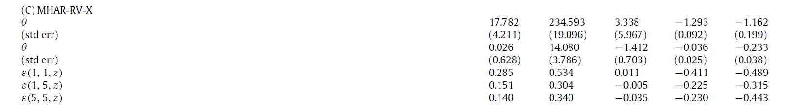 短期利率或信用价差的提升会导致协方差矩阵increase，scorecard以及dividend yield上升则会导致。term structure斜率较小。

 4D展示了含有所有变量模型的弹性。包含滞后波动率后，很多变量的弹性几近消失。

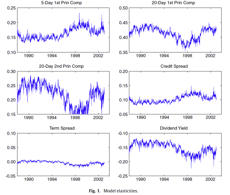
 尽管平均及拟合的弹性展示：特定变量对波动率的较大影响。我们也对弹性的时间序列进行分析。图1展示了六个预测变量的弹性时间序列。三个主成分：滞后5天项的第一主成分、滞后20天项的第一、二主成分，其弹性的时间序列都展示了部分波动。

 5、Conclusion

本文提供一种新的模型，对收益率的已实现协方差矩阵建模。该模型是parsimonious（burden比较小），保证正定协方差矩阵，并且没有参数constraints。

该模型允许多个预测变量预测协方差矩阵，但是从中提取了少数因子。并且，通过预测变量对已实现协方差矩阵的影响，计算了时变的弹性。

该模型应用日度已实现收益率的协方差矩阵，检验了4种模型。已实现周度、月度bi-power协方差滞后项的主成分具有较强预测能力。一些能够预测预期收益的变量也能够预测横截面波动率。所拟合的弹性展示了某些变量的影响是时变的，而某些变量的影响更加稳定。

6、一些思考：

（1）用bi-power covariation对多维波动率建模，实际应用中似乎效果不佳，我们将从HAR模型着手构建潜因子模型；

（2）本文的潜因子思路还是很具有参考价值的，比如对滞后波动率的PCA，结合其他预测变量对高维波动率进行预测，后续潜因子的模型可以参照。