机器学习专栏（46）：高斯混合模型与异常检测（附完整代码与工业级案例）

Sonal_Lynn

已于 2025-05-01 20:30:22 修改

阅读量299

点赞数 3

分类专栏：人工智能专题文章标签：机器学习人工智能算法 python 深度学习神经网络

于 2025-05-01 19:57:01 首次发布

本文链接：https://blog.csdn.net/Conan_0728/article/details/147654191

版权

一、高斯混合模型的核心原理

1.1 概率生成过程解析

1.2 EM算法迭代过程

二、Scikit-Learn实战：从基础到进阶

一、高斯混合模型的核心原理

1.1 概率生成过程解析

给定数据集X，GMM假设数据由k个高斯分布混合生成：

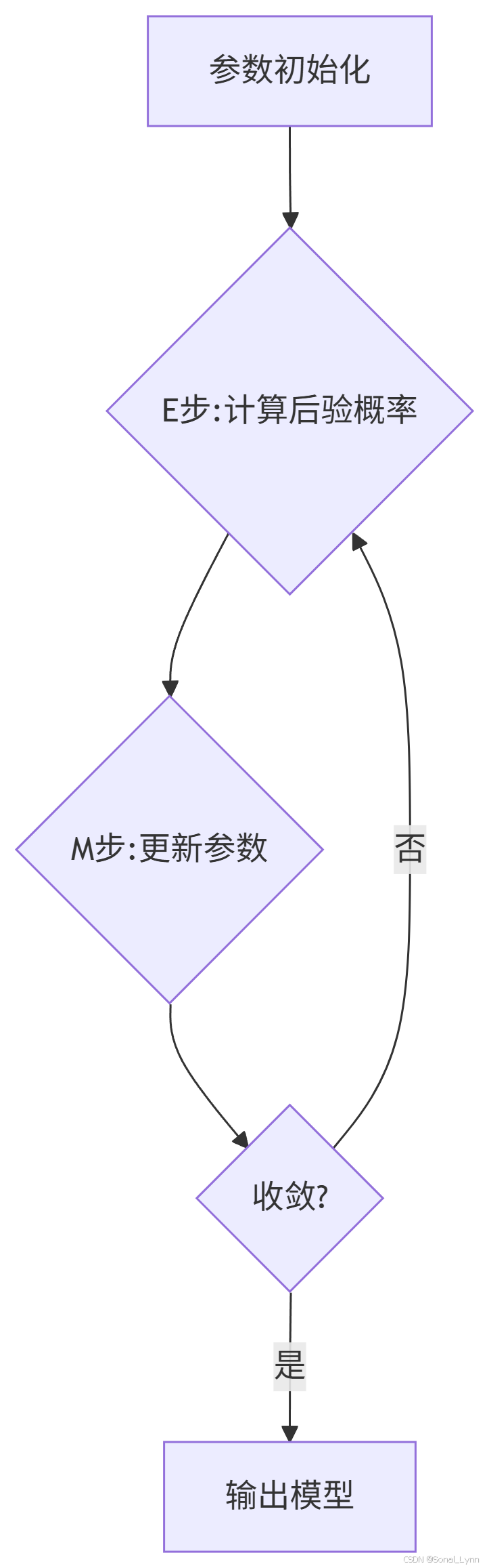
1.2 EM算法迭代过程

二、Scikit-Learn实战：从基础到进阶

2.1 基础建模与可视化

from sklearn.mixture import GaussianMixture
import matplotlib.pyplot as plt
import numpy as np

# 生成模拟数据
np.random.seed(42)
X1 = np.random.normal(0, 1, (300, 2))
X2 = np.random.normal(5, 1.5, (700, 2))
X = np.vstack([X1, X2])

# 训练GMM模型
gmm = GaussianMixture(n_components=2, covariance_type='full')
gmm.fit(X)

# 可视化决策边界
x_min, x_max = X[:,0].min()-1, X[:,0].max()+1
y_min, y_max = X[:,1].min()-1, X[:,1].max()+1
xx, yy = np.meshgrid(np.linspace(x_min, x_max, 100),
                     np.linspace(y_min, y_max, 100))
Z = -gmm.score_samples(np.c_[xx.ravel(), yy.ravel()])
Z = Z.reshape(xx.shape)

plt.contourf(xx, yy, Z, levels=20, cmap='viridis')
plt.scatter(X[:,0], X[:,1], s=5, c='white')
plt.title("GMM概率密度分布")
plt.colorbar(label='负对数概率密度')

2.2 协方差类型对比实验

cov_types = ['spherical', 'tied', 'diag', 'full']
plt.figure(figsize=(15,10))

for i, cov_type in enumerate(cov_types):
    gmm = GaussianMixture(n_components=2, covariance_type=cov_type)
    gmm.fit(X)
    
    # 获取椭圆参数
    if cov_type == 'spherical':
        widths = heights = 2 * np.sqrt(gmm.covariances_)
    else:
        from scipy.stats import multivariate_normal
        widths, heights = [], []
        for cov in gmm.covariances_:
            v, _ = np.linalg.eigh(cov)
            widths.append(2*np.sqrt(v[0]))
            heights.append(2*np.sqrt(v[1]))
    
    plt.subplot(2,2,i+1)
    plt.scatter(X[:,0], X[:,1], s=5, c=gmm.predict(X))
    for j in range(len(gmm.means_)):
        plt.gca().add_patch(plt.Ellipse(gmm.means_[j], widths[j], heights[j], 
                                      angle=0, alpha=0.3))
    plt.title(f'Covariance Type: {cov_type}')

三、工业级异常检测实战

3.1 信用卡欺诈检测

from sklearn.preprocessing import RobustScaler
from sklearn.metrics import classification_report

# 数据预处理
scaler = RobustScaler()
X_trai

最低0.47元/天解锁文章