Deep Temporal Linear EncodingNetwork[Paper & Summary Part]

1. (1)Present a new video representation, called temporal linear encoding (TLE)
   (2)Embedded inside of CNNs as a new layer,which captures the appearance and motion throughout entire videos.
   
2. Encodes this aggregated information into a robust video feature representation, via end-to-end learning.
3. Advantages:
   (1)they encode the entire video into a compact feature representation, learning the semantics and a discriminative feature space
   (2)they are applicable to all kinds of networks like 2D and 3D CNNs for
   video classification
   (3)they model feature interactions in a more expressive way and without loss of information
4. Experiments on HMDB51 (71.1%) & UCF101 (95.6%)
5. TLE is a form of temporal aggregation of features sparsely
   (1)sampled over the whole video using feature map aggregation techniques
   and then (2)projected to a lower dimensional feature space using encoding methods powered by end-to-end learning of deep networks
6. TLE captures the important concepts from the long range temporal structure in different frames or clips, and aggregates it into a compact and robust feature representation by linear encoding.
7. Captures more expressive interactions between the segments across entire videos, and encodes these interactions into a compact representation for video-level prediction.
8. The first end-to-end deep network that encodes temporal features from entire videos
9. Our goal is to create a single feature space in which to represent each video using all its selected frames or clips, rather than scoring separate frames/clips with classifiers and label the video based on scores aggregation.
10. TLE to aggregate spatial and temporal information from an entire video, and to encode it into a robust and compact representation, using end-to-end learning
    
    
    
11. The steps of the proposed TLE
    
    （1）把一段视频切割成K段
    （2）让每一段通过一个CNN，分别提取CNN的features，然后用一个融合操作把它们糅合成一个features，最后进行编码从而得到最终的video representation
12. Different functions T for the temporal aggregation of the segments
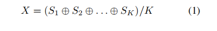
    （1）Element-wise Average of Segments：
    
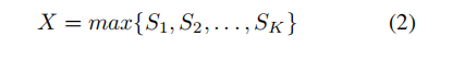
    （2）Element-wise Maximum of Segments：
    
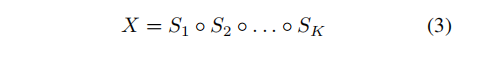
    （3）Element-wise Multiplication of Segments（best results）:
    
13. Encoding methods E
    （1）Bilinear Models： computes the outer product of two feature maps
    
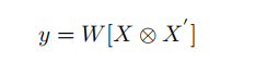
    X ∈ R^(hw)×c & X’∈ R^(hw)×c’ 是输入的两张feature maps
    y ∈ R^cc’是双线性特征
    ⊗ 表示做外积
    [ ] turns the matrix into a vector by concatenating the columns
    W 是模型的参数，是需要通过学习得到的，这里使用的参数是线性的
    在TLE中，X=X’
    The resulting bilinear features capture the interaction of features with each other at all spatial locations, hence leading to a high-dimensional representation. For this reason, we use the Tensor Sketch algorithm，which projects this high-dimensional space to a lower-dimensional space, without computing the outer product directly. That cuts down on the number of model parameters significantly. （降维）
    The model parameters W are learned with end-to-end back propagation.
    （2）Fully connected pooling：
    The network has fully connected layers between the last convolutional layer and the classification layer
    （3）Conclusion
    Bilinear models:
    Projects the high dimensional feature space to a lower dimensional space, which is far fewer in parameters and still perform better than fully-connected layers in performance, apart from computational efficiency.
    Used the features are passed through a signed squared root and L2-normalization.
    Use softmax as a classifier
14. The forward and backward passes
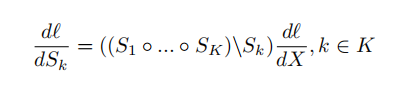
    (1)The Back-propagation for the joint optimization of the
    K temporal segments can be derived as:
    
    (2) The model parameters for the K temporal segments are optimized using stochastic gradient descent (SGD)
    (3) The temporal linear encoding model parameters are learned from the entire video
    (4)Computing gradients for back-propagation
    

15. Implementation details of Two-stream ConvNets

(1)About the Two-stream ConvNets：

(i) The two-stream network consists of spatial and temporal networks, the spatial ConvNet operates on RGB frames, and the temporal ConvNet operates on a stack of 10 dense optical flow frames.
(ii) The input RGB image or optical flow frames are of size 256 × 340, and are randomly cropped to a size 224 × 224, and then mean-subtracted for network training

(2) Fine-tune：

(i) Replace the previous classification layer with a C-way softmax layer, where C is the number of action categories.
(ii) Use mini-batch stochastic gradient descent (SGD) to learn the model parameters with a fixed weight decay of 5 × 10⁻⁴ , momentum of 0.9, and a batch size of 15 for network training
(iii) The prediction scores of the spatial and temporal ConvNets are combined in a late fusion approach as averaging before softmax normalization.

(3)TLE with Bilinear Models：

(i) Retain only the convolutional layers of each network
(ii) Remove all the fully connected layers
(iii) The convolutional feature maps extracted from the last convolutional layers are fed as input into the bilinear models.
(3.1) spatial ConvNets：
Initialize the learning rate with 10⁻³ and decrease it by a factor
of 10 every 4,000 iterations.The maximum number of iterations is set to 12,000.
(3.2)temporal ConvNet：
Use a stack of 10 optical flow frames as input clip
Rescale the optical flow fields linearly to a range of [0, 255] and compress as JPEG images
Initialize the learning rate with 10⁻³ and manually decrease by a factor of 10 every 10,000 iterations. The maximum number of iterations is set to 30,000.
(3.3) Extraction of the optical flow frames Use the TVL1 optical flow algorithm
(3.4) We use batch normalization.
(3.5) Before the features are fed into the softmax layer, the features are passed through a signed squared root operation

(4)TLE with Fully-Connected Pooling:

(4.1) we initialize the learning rate with 10⁻³ and decrease it by a factor of 10 every 10,000,iterations in both model training steps. The maximum number of iterations is set to 30,000.

(5)Aggregation Function:

Three aggregations functions:
(i) element-wise average
(ii)element-wise maximum
(iii) element-wise multiplication(choose)

(6)ConvNet Architectures:

Compare the different ConvNet architectures for TLE:
(i) AlexNet
(ii) VGG-16
(iii)BN-Inception(choose)

(7)Compare the performance of TLE with the current methods using two-stream ConvNets and other traditional methods

(8)Testing:

(i) Divide the given video into 3 parts of equal duration.
(ii) Extact 1 RGB frame or 10 optical flow frames from each part and feed these into the 3 segments network sequentially.
(iii) In total, we sample 5 RGB frames or stacks of
optical flow frames from the whole video.
(iv) Prediction scores of the spatial and temporal ConvNets are
combined in a late fusion approach via averaging.

16. Implementation details of C3D ConvNets

(1) About the C3D ConvNets：

(i) Pre-trained on the Sport-1M dataset.
(ii) The convolution kernels are of size 3×3×3 with stride 1 in both spatial and temporal dimensions.
(iii) The video is decomposed into non-overlapping, equal-duration clips of 16 frames.
(iv) The video frames are of size 128 × 171.
(v) For network training, we randomly crop the video clips to a size 16 × 112 × 112, and then mean-subtract.
(vi) Use a single center crop per clip.

(2) Fine-tune：

(i) Replace the previous classification layer with a C-way softmax layer, where C is the number of action categories.
(ii) Use mini-batch stochastic gradient descent to learn the model parameters with a fixed weight decay of 5 × 10⁻⁴ , momentum of 0.9, and a batch size of 10 for network training

(3)TLE with Bilinear Models：

(i) Retain the convolutional layers.
(ii) Initialize the learning rate with 3 × 10⁻³ and decrease by a factor of 10 every 10,000 iterations. The maximum number of iterations is set to 30,000.
(iii) Use batch normalization
(iv) Before feeding the features to the softmax classifier, the features are passed through a signed squared root and L2-normalization.

(4)TLE with Fully-Connected Pooling:

(i) Initialize the learning rate with 10⁻³ and manually decrease by a factor of 10 every 10,000 iterations. The maximum number of iterations is set
to 40,000.

(5)Testing:

(i) Decompose each video into non-overlapping clips of 16 frames, we then divide the number of clips into 3 equal parts.
(ii) 1 clip is extracted from each part and fed sequentally into the 3 segment network.
(iii) In total, we extract 3 clips from the whole video
(iv) Average the predictions over all groups of clip segments to make a video-level prediction.

(6)Aggregation Function:

Three aggregations functions:
(i) element-wise average
(ii)element-wise maximum
(iii) element-wise multiplication(choose)

(7)Compare the performance of TLE with the current methods using tC3D ConvNets and other traditional methods

17. Conclusion
    (1)Proposed Temporal Linear Encoding (TLE) embedded inside ConvNet architectures, aiming to aggregate information from an entire video, be it in form of frames or clips.
    (2)The model performs action prediction over an entire video.
    (3)computationally efficient, robust, compact, reduce the number of model parameters significantly below that of fully connected ConvNets, and retain the feature interaction in a more expressive way without an undesired loss of information.
    (4)TLEs are flexible enough to be readily employed to other forms of sequential data streams for feature embedding.