吴恩达老师机器学习第一次作业：线性回归【python实现】

【写在前面】

最近刚刚学了python，用来写了下吴恩达老师机器学习第一次作业，没有用别人写好的框架，地址是：

https://github.com/Europe233/ml_homework_py/tree/master/exercise1

【结果展示】

首先给出单变量下的拟合效果：

 

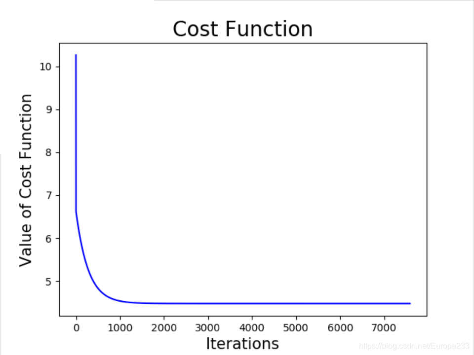
梯度下降法和 Normal Equation 方法结果对比：

 

多变量拟合：

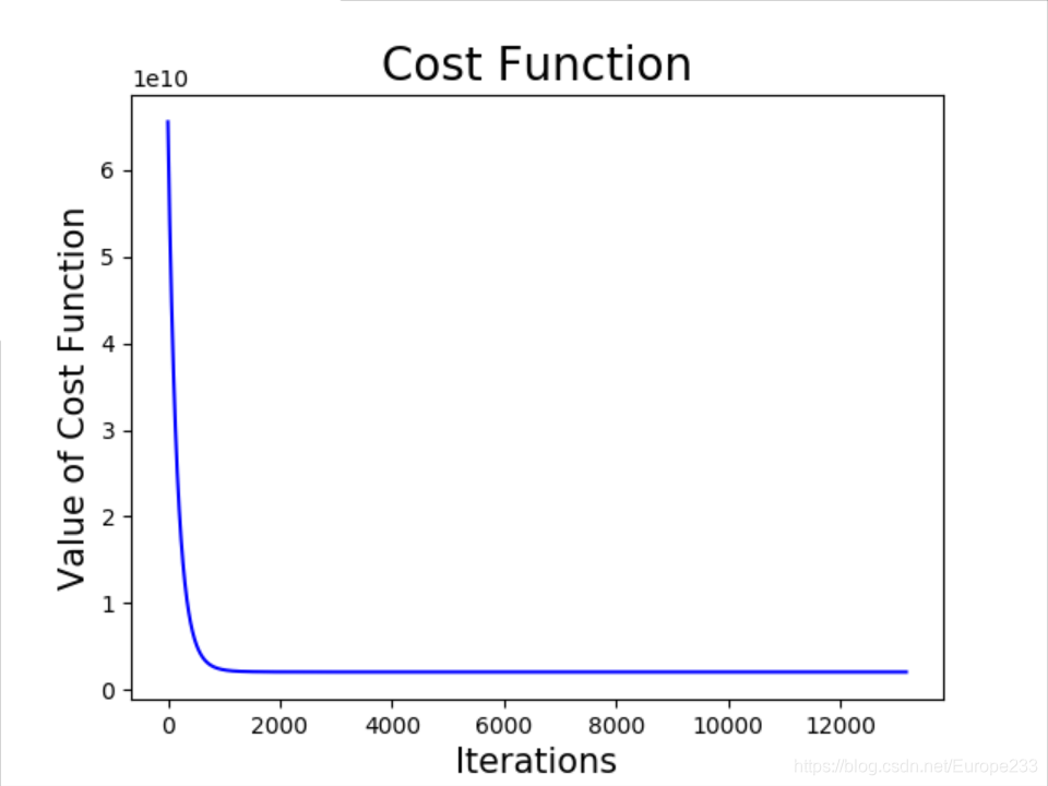
梯度下降法和 Normal Equation 方法结果对比：

 

【代码】

gradientDescent.py

import numpy as np

def gradient_theta(theta,x,y):
    """返回参数的梯度（其反方向即为下一步迭代的搜索方向）"""
    m=y.size

    gra_theta = np.dot(np.dot(theta.T,x.T),x) - np.dot(y.T,x)
    gra_theta = gra_theta/m

    return gra_theta

def next_parameter(alpha,theta,x,y):
    """返回下一步的参数theta"""
    #样本数
    m = y.size

    #参数迭代
    new_theta=theta-alpha*gradient_theta(theta,x,y)
    
    return new_theta

def gradient_descent(alpha,ini_theta,maxIteration,acceptable_err,x,y):
    """从初始参数开始迭代，返回一个列表，记录迭代过程中每一步的参数theta"""
    theta_list = []
    theta_list.append(ini_theta)

    #梯度下降
    while True:
        cnt_theta = theta_list[-1]
        next_theta = next_parameter(alpha,cnt_theta,x,y)
        theta_list.append(next_theta)

        #结束条件：超过最大迭代次数 or 误差可接受
        if np.linalg.norm(gradient_theta(next_theta,x,y))<acceptable_err:
            print("迭代次数：",len(theta_list))
            break
        if len(theta_list) > maxIteration:
            print("迭代次数过多！")
            break

    return theta_list

computeCost.py 

import numpy as np

def  cost(theta,x,y):
    """计算对应参数的Cost"""
    #数据集样本数
    m = y.size

    #计算cost
    err_vec = np.dot(x,theta)-y
    cost = np.dot(err_vec,err_vec)/(2*m)

    return cost

 normalEqn.py

import numpy as np

def normal_eqn(x,y):
    #用normal equation求解theta
    theta = np.linalg.inv(np.dot(x.T,x)).dot(x.T).dot(y)
    
    return theta

plotData.py 

import numpy as np
import matplotlib.pyplot as plt

from computeCost import *

def plot_regression(theta,x,y):
    """根据参数画出拟合的直线"""
     #画出散点图
    plt.scatter(x[:,1],y,c='red',edgecolors='none',s=10)

    #坐标轴设置
    plt.title('Linear Regression',fontsize=20)
    plt.xlabel('Population of City in 10,000s',fontsize=15)
    plt.ylabel('Profit in $10,000s',fontsize=15)

    #画出拟合直线
    line_x = np.linspace(0,25,100)
    line_x = np.c_[np.ones(100),line_x]
    line_y = np.dot(line_x,theta)
    plt.plot(line_x[:,1],line_y,'b')


def plot_cost_descent(theta_list,x,y):
    n = len(theta_list)

    cost_list = []
    for theta in theta_list:
        cnt_cost = cost(theta,x,y)
        cost_list.append(cnt_cost)
    
    x = list(range(n))
    plt.plot(x,cost_list,'b')
    plt.title('Cost Function',fontsize=20)
    plt.xlabel('Iterations',fontsize=15)
    plt.ylabel('Value of Cost Function',fontsize=15)

ML_ex1.py 

import numpy as np
import matplotlib.pyplot as plt

from plotData import *
from gradientDescent import *
from normalEqn import *

#加载数据
data = np.loadtxt('ex1data1.txt',delimiter=',',usecols=(0,1))
x = data[:,0]
y = data[:,1]

m = y.size

x = np.c_[np.ones(m),x] #加上一列1到x

#初始参数,学习率,可接受误差，最大迭代次数
ini_theta = np.array([1.0,1.0])
alpha = 0.01
acceptable_err = 1e-6
maxIteration = 10000

#梯度下降
theta_list = gradient_descent(alpha,ini_theta,maxIteration,acceptable_err,x,y)

#比较梯度下降和normal equation的解
print('梯度下降最终结果：    theta = ',theta_list[-1])
print('Normal Equation结果： theta = ',normal_eqn(x,y))

# 可视化
plot_regression(theta_list[-1],x,y)
plt.show()
plot_cost_descent(theta_list,x,y)
plt.show()

多变量：

featureNormalize.py

import numpy as np

def feature_normalize(x):
    """对数据集做 normalization : avg返回各个feature的均值，std返回各个feature的标准差...
    ...normalized_x 返回normalize后的x"""

    #获取featrue个数 n
    n = x.shape[1]

    #计算 avg，std
    avg = np.mean(x,axis=0)
    std = np.std(x,axis=0)

    #计算 noramlized_x
    normalized_x = x.copy()
    for i in range(n):
        #对第 i 个feature进行处理
        normalized_x[:,i] = (x[:,i]-avg[i])/std[i]

    return avg,std,normalized_x

ML_ex1_multi.py 

import numpy as np

from featureNormalize import *
from gradientDescent import *
from plotData import *
from normalEqn import *

#读入数据
data = np.loadtxt('ex1data2.txt',delimiter=',')

x = data[:,0:2]
y = data[:,2]

m = y.size   #获取样本数
n = x.shape[1]  #feature个数

# Normalization
avg,std,x = feature_normalize(x)

x = np.c_[np.ones(m),x] #加上一列1到x上

#初始参数,学习率,可接受误差，最大迭代次数
ini_theta = np.zeros(n+1)
alpha = 0.003
maxIteration = 100000
acceptable_err = 1e-3

#梯度下降
theta_list = gradient_descent(alpha,ini_theta,maxIteration,acceptable_err,x,y)

##比较梯度下降和normal equation的解
print('梯度下降最终结果：    theta = ',theta_list[-1])
print('Normal Equation结果： theta = ',normal_eqn(x,y))

#可视化
plot_cost_descent(theta_list,x,y)
plt.show()

 

 

【个人总结】

虽然是很简单的实现，但还是有所收获：

0.学习率 alpha 固定在应用时并不好用，首先过大会不收敛，过小太慢。这时候才知道凸优化中的 back line search 真是非常有用的方法！

 

1. 在实现过程里面，出现了一个bug，后面发现问题是这样的：我初始化一个array时，用的语句是：

ini_theta = np.array([0,0])

然后这个array里的数就是 int 类型的，参与之后的浮点数运算就出了问题，后来改成了：

ini_theta = np.array([0.0,0.0])

 

2. 一个小小的发现是：一边运算一边用print语句把东西输出到终端非常耗时

 

3.把一个array(设为a)赋给一个变量，这个变量实际类似于C++里的引用(reference)，如果不想这样可以用 a.copy()

 

4. python中的切片，结束的下标不会出现在结果里。例如 a = [1,2,3]，那么 a[0:2] 就是 [1,2]