机器学习技法 之 径向基函数网络（RBF Network）

径向基函数网络（Radial Basis Function Network）：就是将基假设函数进行线性聚合。

径向基函数网络假设函数（RBF Network Hypothesis）

先回顾一下高斯支持向量机（Gaussian SVM）：

$$g_{\mathrm{s}\mathrm{v}\mathrm{m}}(\mathbf{x})=\mathrm{sign}\left(\sum _{\mathrm{S}\mathrm{V}}{\alpha }_n{y}_n\exp \left(-\gamma {\Vert \mathbf{x}-{\mathbf{x}}_n\Vert }^2\right)+b\right)$$

其实际上是找出系数 ${\alpha }_n$ 将以 ${\mathbf{x}}_n$ 为中心的高斯函数进行线性结合。

Gaussian kernel 又叫 Radial Basis Function (RBF) kernel，其中 Radial 指的是这里之关系 $\mathbf{x}$ 与中心 ${\mathbf{x}}_n$ 之间的距离（类似于一种放射线长度求解）。

那么写出高斯支持向量机中的径向基假设函数：

$$g_n(\mathbf{x})=y_n\exp \left(-\gamma {\Vert \mathbf{x}-{\mathbf{x}}_n\Vert }^2\right)$$

那么高斯支持向量机可以改写为：

$$g_{\mathrm{s}\mathrm{v}\mathrm{m}}(\mathbf{x})=\mathrm{sign}\left(\sum _{\mathrm{S}\mathrm{V}}{\alpha }_n{g}_n(\mathbf{x})+b\right)$$

可以看出被选择的径向基假设函数的线性结合（linear aggregation of selected radial hypotheses）。

RBF Network 的网络结构示意图如下：

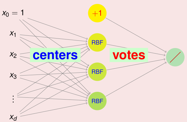
实际上 RBFNet 是 NNet 的一个分支，可见输出层虽然使用的是投票，但是这也是一种线性组合所以与神经网络是一样的。但是隐含层是不同的，在神经网络中使用的是内积加 tanh 输出，而在 RBFNet 中使用的是距离计算加高斯函数。

那么可以写出 RBFNet 的输出假设函数：

$$h(\mathbf{x})=\text{ Output }\left(\sum _{m=1}^M{\beta }_m\mathrm{RBF}\left(\mathbf{x},{\mu }_m\right)+b\right)$$

其中 ${\mu }_m$ 是中心点，${\beta }_m$ 是投票系数。

对比与高斯支持向量机：

1. RBF（径向基函数）选择的是高斯函数。
2. Output（输出）选择 sign 做为二分类输出。
3. M 则是支持向量的个数（#SV）。
4. ${\mu }_m$ 则是支持向量 ${\mathbf{x}}_m$。
5. ${\beta }_m$ 则是通过 SVM Dual 问题求解 ${\alpha }_m$ 与 $y_m$ 的乘积。

不失普遍性的来说：如果要学习径向基函数网络的话，需要选择四个部分：径向基函数 RBF ，输出层假设函数 Output ，中心点的求取 ${\mu }_m$ ，投票的系数 ${\beta }_m$。

实际上核技巧实际上就是根据在 $\mathcal{Z}$ 空间上的内积求取相似性，比如多项式核：

$$\mathrm{Poly}\left(\mathbf{x},{\mathbf{x}}^{\prime }\right)={\left(1+{\mathbf{x}}^T{\mathbf{x}}^{\prime }\right)}^2$$

而RBF则是直接通过在 $\mathcal{X}$ 空间上的距离求取相似性，一般认为距离越近相似性越大，也就是说距离与相似性单调相关。比如下面这个截断相似性函数：

$$\text{ Truncated }\left(\mathbf{x},{\mathbf{x}}^{\prime }\right)=\left[\Vert \mathbf{x}-{\mathbf{x}}^{\prime }\Vert \le 1\right]{\left(1-\Vert \mathbf{x}-{\mathbf{x}}^{\prime }\Vert \right)}^2$$

而高斯函数则处于他们的交集。

$$\text{ Gaussian }\left(\mathbf{x},{\mathbf{x}}^{\prime }\right)=\exp \left(-\gamma {\Vert \mathbf{x}-{\mathbf{x}}^{\prime }\Vert }^2\right)$$

相似性是很好的一种特征转换方法。在RBF中则是将中心距离相似性作为特征转换的。其他的相似性函数比如神经元函数或者DNA序列相似性函数：

$$\begin{array}{c}\text{ Neuron }\left(\mathbf{x},{\mathbf{x}}^{\prime }\right)=\tanh \left(\gamma {\mathbf{x}}^T{\mathbf{x}}^{\prime }+1\right)\\ \text{ DNASim }\left(\mathbf{x},{\mathbf{x}}^{\prime }\right)=\text{ EditDistance }\left(\mathbf{x},{\mathbf{x}}^{\prime }\right)\end{array}$$

RBF网络的训练/学习（RBF Network Learning）

完全RBF网络（Full RBF Network）

如果不考虑 bais ，那么可以写为：

$$h(\mathbf{x})=\mathrm{Output}\left(\sum _{m=1}^M{\beta }_m\mathrm{RBF}\left(\mathbf{x},{\mathbf{\mu }}_m\right)\right)$$

如果令 $M=N$ 并且每一个 ${\mu }_m={\mathbf{x}}_m$ 那么这个RBF网络便是完全RBF网络（full RBF Network）。这么做的物理意义是 ${\mathbf{x}}_m$ 将通过系数 ${\beta }_m$ 来影响每一个与之相似的 $\mathbf{x}$。

那么举例来说，如果使用一个 uniform influence 即 ${\beta }_m=1\cdot y_m$，也就是说大家票数一致。

$$g_{\text{unitorm }}(\mathbf{x})=\mathrm{sign}\left(\sum _{m=1}^N{y}_m\exp \left(-\gamma {\Vert \mathbf{x}-{\mathbf{x}}_m\Vert }^2\right)\right)$$

所以说完全RBF网络是一种偷懒的做法，省去了中心向量 ${\mu }_m$ 的求取。

最邻近算法（Nearest Neighbor）

由于高斯函数衰减很快，那么会导致离中心最近的值会获得很大的权重，支配（dominates）投票过程，也就是说具有 “专断权”。所以这个过程更类似于选择一个最大值（最近向量），而不是聚合过程。即：

$$g_{\text{nbor }}(\mathbf{x})=y_m\text{ such that }\mathbf{x}\text{ closest to }{\mathbf{x}}_m$$

所以叫做最邻近模型（nearest neighbor model）。

常用的是 K 邻近模型，根矩 Top k 最邻近的样本进行均值投票（uniformly aggregate k neighbor），虽然很懒（lazy）但是很直观。

无正则化用于插值（Interpolation）

那么如果用于 Regression，那么以平方误差作为误差测量函数，最后的假设函数可以写为：

$$h(\mathbf{x})=\left(\sum _{m=1}^N{\beta }_m\mathrm{RBF}\left(\mathbf{x},{\mathbf{x}}_m\right)\right)$$

可以看出这就是在通过 RBF 映射到的空间上训练线性回归模型

那映射后的数据表示为：

$${\mathbf{z}}_n=\left[\mathrm{RBF}\left({\mathbf{x}}_n,{\mathbf{x}}_1\right),\mathrm{RBF}\left({\mathbf{x}}_n,{\mathbf{x}}_2\right),\dots ,\mathrm{RBF}\left({\mathbf{x}}_n,{\mathbf{x}}_N\right)\right]$$

矩阵 $\mathrm{Z}$ 由 $n$ 个 ${\mathbf{z}}_n$ 构成，所以矩阵 $\mathrm{Z}$ 为 $N\text{(example)}\times N\text{(centers)}$ 的对称方阵（symmetric square matrix），根据线性回归可以写出 $\beta$ 的最优解：

$$\beta ={\left({\mathrm{Z}}^T\mathrm{Z}\right)}^{-1}{\mathrm{Z}}^T\mathbf{y},\text{ if }{\mathrm{Z}}^T\mathrm{Z}\text{ invertible }$$

那么如果全部的 ${\mathbf{x}}_n$ 的都是不同的，那么 $\mathrm{Z}$ （with Gaussian RBF）便是可逆的（invertible）。

又因为 $\mathrm{Z}$ 是对称方阵，也就是说 ${\mathrm{Z}}^T=\mathrm{Z}$。那么可以化简为：

$$\beta ={\left(\mathrm{Z}\mathrm{Z}\right)}^{-1}\mathrm{Z}\mathbf{y}={\mathrm{Z}}^{-1}\mathbf{y}$$

正则化（Regularization）

那么 ${\mathrm{x}}_1$ 的 RBF的网络输出为：

$$g_{\mathrm{R}\mathrm{B}\mathrm{F}}\left({\mathrm{x}}_1\right)={\mathbf{\beta }}^T{\mathrm{z}}_1={\mathbf{y}}^T{\mathrm{Z}}^{-1}(\text{first column of }\mathrm{Z})={\mathbf{y}}^T{\left[\begin{array}{llll}1& 0& \dots & 0\end{array}\right]}^T=y_1$$

也就是说 $g_{\mathrm{R}\mathrm{B}\mathrm{F}}\left({\mathrm{x}}_n\right)=y_n,\text{ i.e. }{E}_{\mathrm{i}\mathrm{n}}\left(g_{\mathrm{R}\mathrm{B}\mathrm{F}}\right)=0$，那么这样的结果用于精确插值的函数估计（exact interpolation for function approximation）是非常好的，但是在机器学习中便会出现过拟合问题。所以可以加入 Regularization，当然前面学习过岭回归（ridge regression），可以将 regularized full RBFNet $\beta$ 的求解改写为：

$$\beta ={\left({\mathrm{Z}}^T\mathrm{Z}+\lambda \mathrm{I}\right)}^{-1}{\mathrm{Z}}^T\mathrm{y}$$

在 kernel ridge regression 中，有一个 $\mathbf{K}$ 矩阵：

$$\mathrm{Z}=\left[\text{Gaussian }\left({\mathbf{x}}_n,{\mathbf{x}}_m\right)\right]=\text{ Gaussian kernel matrix }\mathbf{K}$$

在 kernel ridge regression 中，$\beta$ 的求解为：

$$\beta =(\mathrm{K}+\lambda \mathrm{I}{)}^{-1}\mathrm{y}$$

两者很相近，但是由于正则化的对象不同所以求解公式也不同，在核岭回归中的针对的正则化对象为无限多维的转换。而 RBF 中针对的是有限多维的 $N$ 维的转换。

K均值算法（k-Means Algorithm）

反观 SVM，实际上并没有使用到全部的 ${\mathbf{x}}_n$ ，而只是用到了支持向量，即 $M\ll N$。

$$g_{\mathrm{s}\mathrm{v}\mathrm{m}}(\mathbf{x})=\mathrm{sign}\left(\sum _{\mathrm{S}\mathrm{V}}{\alpha }_m{y}_m\exp \left(-\gamma {\Vert \mathbf{x}-{\mathbf{x}}_m\Vert }^2\right)+b\right)$$

也就是通过限制中心的个数和投票的权重来达到正则化的效果（regularization by constraining number of centers and voting weights）。

现在的思路是找出一些“中心”代表（prototypes）。

聚类问题（Clustering Problem）

找代表的过程实际上是一种聚类问题。什么意思呢？

$$\begin{array}{l}\text{ if }{\mathbf{x}}_1\approx {\mathbf{x}}_2\\ ⟹\text{ no need both }\mathrm{RBF}\left(\mathbf{x},{\mathbf{x}}_1\right)\&\mathrm{RBF}\left(\mathbf{x},{\mathbf{x}}_2\right)\text{ in RBFNet }\\ ⟹\text{ cluster }{\mathbf{x}}_1\text{ and }{\mathbf{x}}_2\text{ by one prototype }\mu \approx {\mathbf{x}}_1\approx {\mathbf{x}}_2\end{array}$$

也就是说 $\mathrm{RBF}\left(\mathbf{x},{\mathbf{x}}_1\right)$ 可以很大程度上代表（表示） $\mathrm{RBF}\left(\mathbf{x},{\mathbf{x}}_2\right)$。

那么这种通过代表（代理人）进行聚类（clustering with prototype）的过程为：

1. 将 { x n } \left\{ \mathbf { x } _ { n } \right\} {xn​} 分为M个互斥（不想交）的集合（disjoint sets）：$S_1,S_2,\cdots ,S_M$。
2. 为每一个 $S_m$ 选择最佳的 ${\mu }_m\approx {\mathbf{x}}_{1_m}\approx \cdots \approx {\mathbf{x}}_{K_m}$ ，其中 ${\mathbf{x}}_{1_m}\cdots {\mathbf{x}}_{K_m}\in S_m$。

使用平方测量的聚类误差

$$E_{\mathrm{i}\mathrm{n}}\left(S_1,\cdots ,S_M;{\mu }_1,\cdots ,{\mu }_M\right)=\frac{1}{N}\sum _{n=1}^N\sum _{m=1}^M\left[{\mathbf{x}}_n\in S_m\right]{\Vert {\mathbf{x}}_n-{\mathbf{\mu }}_m\Vert }^2$$

所以现在的聚类问题的优化目标为：

min ⁡ { S 1 , ⋯   , S M : μ 1 , ⋯   , μ M } E i n ( S 1 , ⋯   , S M ; μ 1 , ⋯   , μ M ) \min _ { \left\{ S _ { 1 } , \cdots , S _ { M } : \mu _ { 1 } , \cdots , \mu _ { M } \right\} } E _ { i n } \left( S _ { 1 } , \cdots , S _ { M } ; \mu _ { 1 } , \cdots , \mu _ { M } \right) {S1​,⋯,SM​:μ1​,⋯,μM​}min​Ein​(S1​,⋯,SM​;μ1​,⋯,μM​)

优化（Optimization）

在优化过程中涉及到两个部分的最佳化问题：如何分群以及如何寻找中心点。

这样的组合和数值（ combinatorial-numerical optimization）两个问题结合优化的过程是比较难以优化的：

那么如果只对一个问题寻优，那么问题就会简单很多。

分区寻优（Partition Optimization）

假设 ${\mu }_1,{\mu }_2,\dots ,{\mu }_k$ 已经固定，那么一个又一个地通过下面这个公式选择最优的组群：

$$\text{ optimal chosen subset }{S}_m=\text{ the one with minimum }{\Vert {\mathbf{x}}_n-{\mathbf{\mu }}_m\Vert }^2$$

也就是对于每一个 ${\mathbf{x}}_n$ 都在 ${\mu }_1,{\mu }_2,\dots ,{\mu }_k$ 中选择最近的 ${\mu }_m$ ，并以此为依据进行最优分区（optimally partitioned）。

代表寻优（Prototype Optimization）

假设 $S_1,\cdots ,S_M$ 已经固定，那么这个优化问题便成为了一个关于每一个 ${\mu }_m$ 的无约束最优化问题：

$${\nabla }_{{\mathbf{\mu }}_m}{E}_{\mathrm{i}\mathrm{n}}=-2\sum _{n=1}^N\left[{\mathbf{x}}_n\in S_m\right]\left[{\mathbf{x}}_n-{\mathbf{\mu }}_m\right)=-2\left(\left(\sum _{{\mathbf{x}}_n\in S_m}{\mathbf{x}}_n\right)-\left|S_m\right|{\mathbf{\mu }}_m\right)$$

可以看出来最优的代表值便是全部样本的平均值：

$$\text{ optimal prototype }{\mu }_m=\text{ average of }{\mathbf{x}}_n\text{ within }{S}_m$$

对于每个 $S_1,S_2,\dots ,S_k$ 都求均值作为最佳 ${\mu }_m$ 的计算方法（optimally computed）。

具体实现

$$\begin{array}{l}\text{ (1) initialize }{\mu }_1,{\mu }_2,\dots ,{\mu }_k:\text{ say, as }k\text{ randomly chosen }{x}_n\\ \text{ (2) alternating optimization of }{E}_{\text{in }}\text{ : repeatedly }\\ \text{ (1) Optimize }{S}_1,S_2,\dots ,S_k:\text{ each }{x}_n\text{ optimally partitioned using its closest }{\mu }_i\\ \text{ (2) Optimize }{\mu }_1,{\mu }_2,\dots ,{\mu }_k\text{ : each }{\mu }_n\text{ optimally computed as the consensus within }{S}_m\\ \text{ until converge }\end{array}$$

收敛（converge ）：$S_1,S_2,\dots ,S_k$ 不再改变。因为上述的交替迭代过程是使得 $E_{\text{in }}$ 不断变小的过程，同时$E_{\text{in }}$ 的最小值为 0，所以必然收敛。

由于交替寻优（alternating minimization）的特性，K均值算法成为了最流行的距离算法。

正则化RBF网络

使用K均值算法，找出K个具有代表性的 ${\mu }_k$，来构造 $N\text{(examples)}\times K\text{(centers)}$ 的 $\mathrm{Z}$ 矩阵。

那么 RBF Network Using k-Means 的实现过程为：

 (1) run  k  -Means with  k = M  to get  { μ m }  (2) construct transform  Φ ( x )  from RBF (say, Gaussian) at  μ m Φ ( x ) = [ RBF ⁡ ( x , μ 1 ) , RBF ⁡ ( x , μ 2 ) , … , RBF ⁡ ( x , μ M ) ]  (3) run linear model on  { ( Φ ( x n ) , y n ) }  to get  β  (4) return  g RBFNET  ( x ) =  LinearHypothesis  ( β , Φ ( x ) ) \begin{array} { l } \text { (1) run } k \text { -Means with } k = M \text { to get } \left\{ \boldsymbol { \mu } _ { m } \right\} \\ \text { (2) construct transform } \Phi ( \mathbf { x } ) \text { from RBF (say, Gaussian) at } \mu _ { m } \\ \qquad \mathbf { \Phi } ( \mathbf { x } ) = \left[ \operatorname { RBF } \left( \mathbf { x } , \mu _ { 1 } \right) , \operatorname { RBF } \left( \mathbf { x } , \mu _ { 2 } \right) , \ldots , \operatorname { RBF } \left( \mathbf { x } , \mu _ { M } \right) \right] \\ \text { (3) run linear model on } \left\{ \left( \mathbf { \Phi } \left( \mathbf { x } _ { n } \right) , y _ { n } \right) \right\} \text { to get } \beta \\ \text { (4) return } g _ { \text {RBFNET } } ( \mathbf { x } ) = \text { LinearHypothesis } ( \boldsymbol { \beta } , \mathbf { \Phi } ( \mathbf { x } ) ) \end{array}  (1) run k -Means with k=M to get {μm​} (2) construct transform Φ(x) from RBF (say, Gaussian) at μm​Φ(x)=[RBF(x,μ1​),RBF(x,μ2​),…,RBF(x,μM​)] (3) run linear model on {(Φ(xn​),yn​)} to get β (4) return gRBFNET ​(x)= LinearHypothesis (β,Φ(x))​

这实际上就是使用无监督学习方法来辅助特征转换（using unsupervised learning (k-Means) to assist feature transform）。需要的参数有两个：一个是代表的个数 $M$，另一个是RBF的选择（比如中心为 $\gamma$ 的高斯函数）。

k-Means和RBF网络的实际应用（k-Means and RBF Network in Action）

K-Means in Action

下面展示k-Means算法的实际优化过程：

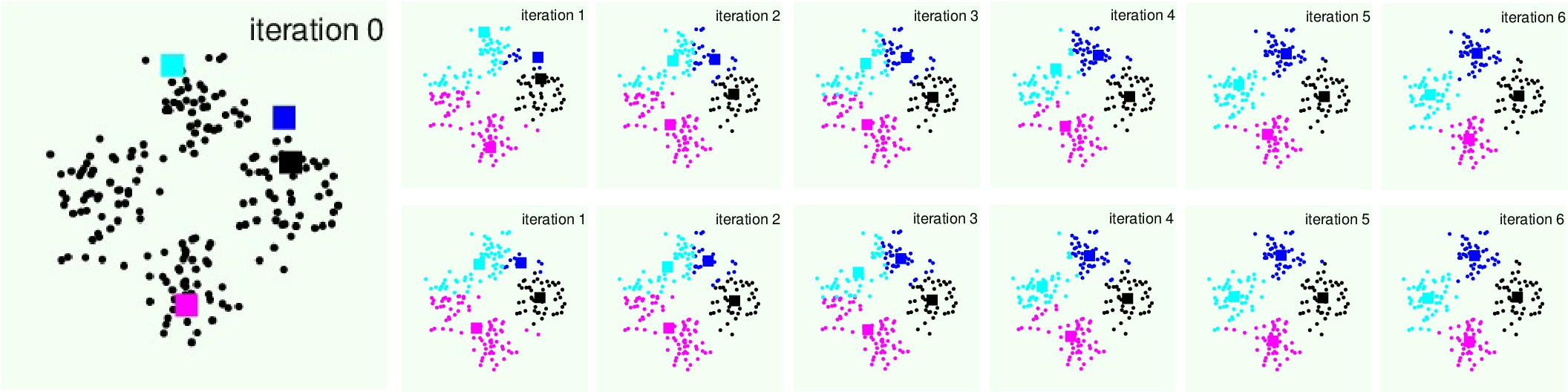
其中第一行是分区优化，第二行是代表（中心点）寻优。可看出合理的初始值和k可以获得不错的聚类效果。

RBF Network Using k-Means in Action

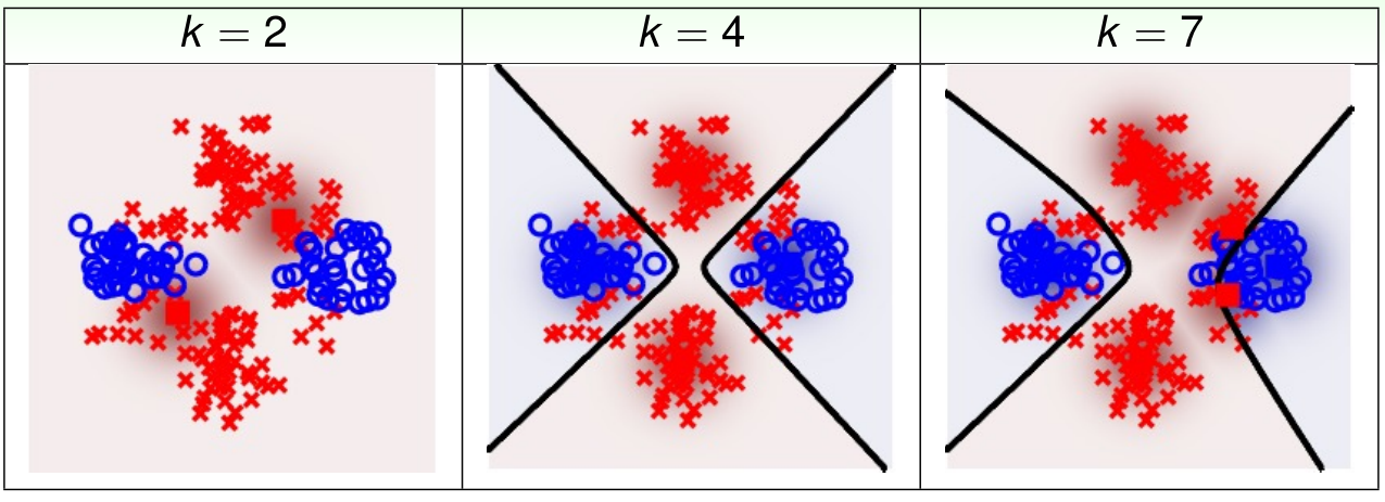
图中发黑的地方代表了高斯密度函数的分布形式。可以看出合理的中心点可以使得 RBF Network 获得比较好的效果。

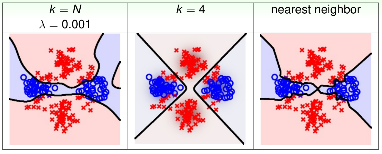
Full RBF Network in Action

最左边是使用了正则化的RBF的分类效果。最右边是最近邻算法的分类效果。因为两者在一定程度上都用到了全部的数据，所以看起来有些过拟合。所以在实际运用中完全 RBF 网络很少使用。