机器学习中的精确率召回率和PR曲线

阈值对精确率和召回率的影响

精确率和召回率是相互矛盾的一组指标，即精确率提高就会导致召回率降低。

假设我有一组样本，分别为蓝色点和红色点，我们想要用算法模型预测出红色点。
当阈值选择在红色分隔线的位置时：
精确率 = 5 / 6 = 0.83
召回率 = 5 / 7 = 0.71

当阈值选择在黑色分割线的位置时：
精确率 = 7 / 10 = 0.7
召回率 = 7 / 7 = 1

当阈值选择在蓝色分割线的位置时：
精确率 = 3 / 3 = 1
召回率 = 3 / 7 = 0.43

由此可见，无法同时增加精准率和召回率，精确率和召回率是相互牵制的一组指标。

在逻辑回归的分类中，当我们预测出的结果大于0，将结果带入sigmoid函数中，模型会判断其为“1”的概率大于0.5，所以就会认为结果为“1”，当预测结果小于0，则sigmoid函数输出结果小于0.5，则预测为“0”

所以0就是逻辑回归中的阈值，红色的线就是一个决策边界。当我们调整阈值就可以调整决策边界，就可以改变我们的分类结果。

下面通过代码来实际看下精确率召回率f1score和阈值之间的关系。
还是使用sklearn里自带的手写识别数据集，还是手工将数据集修改为二分类问题，把结果为9的置为1，结果为其他数字的置为0。然后训练逻辑回归模型。

from sklearn import datasets
import numpy as np
import matplotlib.pyplot as plt
from sklearn.linear_model import LinearRegression,LogisticRegression
from sklearn.model_selection import train_test_split

digits = datasets.load_digits()
X = digits.data
y = digits.target.copy()
y[digits.target == 9] = 1
y[digits.target != 9] = 0
X_train, X_test, y_train, y_test = train_test_split(X, y, test_size=0.25, random_state=666)

log_reg = LogisticRegression() #构建逻辑回归模型
log_reg.fit(X_train,y_train) #使用训练数据集训练模型
y_predict = log_reg.predict(X_test) #将测试数据传入训练好的模型中，让模型预测测试数据的结果

在默认逻辑回归中，0为该模型的阈值，如果分数>0这被分为“1”类，如果分数<0,则被分为“0”类。可以用decision_function方法来看逻辑回归中每个样本的分数。

我们写一个for循环，不断改变threshold阈值，在不同阈值下算出对应的精准率召回率和f1score值。

from sklearn.metrics import confusion_matrix,precision_score,recall_score,f1_score

decision_scores = log_reg.decision_function(X_test) #找到每个样本在这个逻辑回归模型中的score值
thresholds = np.arange(np.min(decision_scores),np.max(decision_scores))
precision_scores,recall_scores,f1_scores = [],[],[]
for threshold in thresholds:
    y_predict_threshold = np.array(decision_scores >= threshold, dtype='int')
    precision_scores.append(precision_score(y_test,y_predict_threshold))
    recall_scores.append(recall_score(y_test,y_predict_threshold))
    f1_scores.append(f1_score(y_test,y_predict_threshold))

plt.plot(thresholds,precision_scores,label='precision_score')
plt.plot(thresholds,recall_scores,label='recall_score')
plt.plot(thresholds,f1_scores,label='f1_score')
plt.legend()
plt.xlabel("thresholds")
plt.grid()
plt.show()

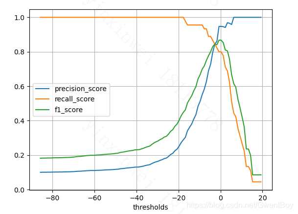
结果如上图所示，我们画出了不同阈值下模型的精确率和召回率的变化趋势，我们在选择模型阈值的时候，可以看这个图，如果想要模型精确率在90%以上，那么阈值就可以在横坐标上进行选择。

精确率-召回率曲线

下面我们画出精确率和召回率的关系图：

plt.plot(precision_scores,recall_scores)

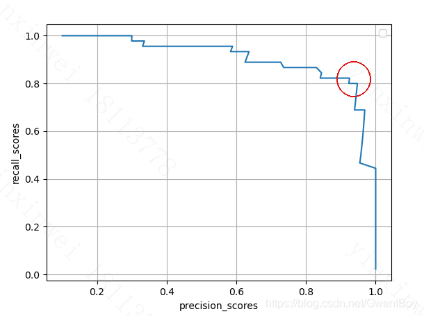
图中可以看出随着精确率上升，召回率是不断下降的。而且图中随着精确率上升，从一个点开始召回率下降的很快，而在这个点之前召回率下降的幅度并不是很明显。这个点就是精确率和召回率比较平衡的位置，在这之前和在这之后精确率和召回率都会有大幅下降。

上文是我们自己实现了precision_recall_curve的方法，其实在sklearn中封装好了precision_recall_curve的方法

from sklearn.metrics import precision_recall_curve
precisions,recalls,thresholds = precision_recall_curve(y_test,decision_scores)

注意：分别打印precisions,recalls,thresholds的shape，发现thresholds的个数比precisions,recalls少一个。

The last precision and recall values are 1. and 0. respectively and do not have a corresponding threshold.  This ensures that the graph starts on the y axis.

所以画图时取precisions,recalls时要剔除最后一个元素。

最后说说这个PR图像的含义。

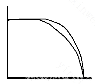
如果有两个算法，或者一个算法用两个不同参数进行训练，训练出的PR图像如上，那么通常曲线与x,y轴相交的面积更大的模型会更好。因为外面这根线对应的模型，每个点的精确率和召回率都更好。