


代码需要的数据,我也无法获取,需要大家自行申请。另外,哪位好心人可以私底下分享给我一份那就非常感谢了。

介绍
Cellular communities reveal trajectories of brain ageing and Alzheimer’s disease 文章提供了完整的代码和数据,可以直接复现单细胞数据分析。虽然它特别适合新手上路,但数据的获取很难,需要经过申请。
图1
source("5. Manuscript code/utils.R")
source("1. Library preprocessing/utils/ROSMAP.metadata.R")
# Loading list of snRNA-seq participants, while correcting mistakes in tracker file
participants <- openxlsx::read.xlsx("5. Manuscript code/data/ROSMAP 10X Processing Tracker.xlsx", sheet = "Processed Batches") %>%
filter(!Batch %in% c("B1", "B2", "B3") & (!StudyCode %in% c("MAP83034844", "MAP74718818"))) %>%
mutate(StudyCode = as.character(as.numeric(gsub("ROS|MAP", "", StudyCode)))) %>%
select(StudyCode, Batch) %>%
rbind(data.frame(StudyCode="44299049", Batch=55))
# The following loads ROSMAP participants' demographic- and endophenotypic characterization
# Parts of these data are available in supplementary table 1
cohort <- load.metadata() %>% `[`(unique(participants$StudyCode), )
#####################################################################################################################
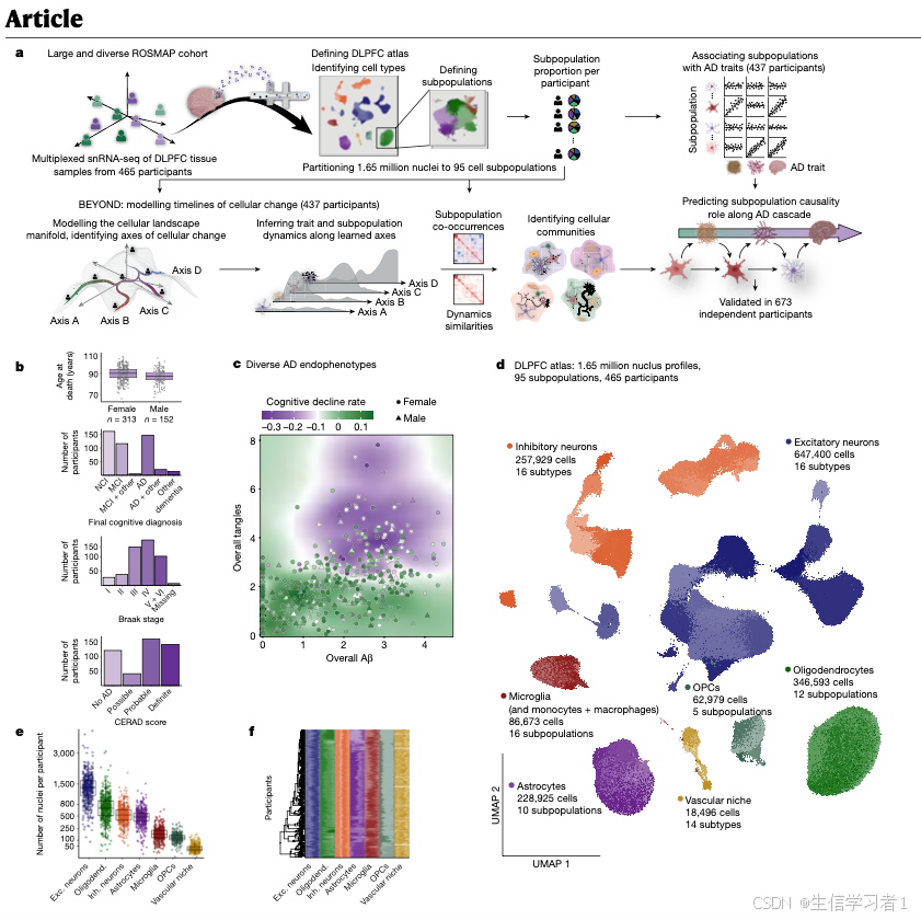
# Figure 1 - Cohort & Atlas Overview #
#####################################################################################################################
# ----------------------------------------------------------------------------------------------------------------- #
# Panel B - Categorical Pathology & Cognitive Decline #
# ----------------------------------------------------------------------------------------------------------------- #
p1 <- ggplot(cohort, aes(sex, age_death)) +
geom_jitter(alpha=.4, width = .15) +
geom_boxplot(alpha=.5, fill="darkorchid4", outlier.size = 0) +
stat_summary(geom = "text", fun.data = function(x) list(y=65, label=paste0("n=", length(x)))) +
labs(x=NULL, y="Age of death", title=NULL) +
scale_y_continuous(breaks = c(70, 90, 110)) +
theme_classic()
pdf(file.path(panel.path, "1B.pdf"), width=embed.width, height=embed.height*2)
plot_grid(p1, plot_grid(plotlist = lapply(c("cogdx.grouped.txt","braak.grouped.txt","cerad.txt"), function(t)
ggplot(cohort, aes(!!sym(t), fill=!!sym(t))) +
geom_bar(color="black") +
theme_classic() +
scale_fill_manual(values = colorRampPalette(c("white","darkorchid4"))(1+length(unique(cohort[,t])))[-1]) +
scale_y_continuous(expand = c(0,0),
limits = c(0, 170),
breaks = c(50,100, 150)) +
labs(x=NULL, y=t, title=NULL)),
ncol=1),
rel_heights = c(1,3), ncol = 1)
while (!is.null(dev.list())) dev.off()
rm(p1)
# ----------------------------------------------------------------------------------------------------------------- #
# Panel C - quantative Pathology & Cognitive Decline #
# ----------------------------------------------------------------------------------------------------------------- #
df <- cohort[,c("sqrt.amyloid","sqrt.tangles","cogng_demog_slope","sex")] %>%
filter(!is.na(sqrt.amyloid) & !is.na(sqrt.tangles)) %>%
rename(x="sqrt.amyloid", y="sqrt.tangles")
grid <- expand.grid(x=seq(-.05, 1.05*max(df$x, na.rm = T), length.out=200),
y=seq(-.05, 1.05*max(df$y, na.rm = T), length.out=200))
dist <- rdist::cdist(grid, df[!is.na(df$cogng_demog_slope),1:2])^2
dens <- apply(dist, 1, function(x) sqrt(mean(sort(x, partial=10)[1:10])))
C <- as.matrix(df[!is.na(df$cogng_demog_slope),"cogng_demog_slope"])
grid$cogng_demog_slope <- exp(-dist/(.75*dens)) %*% C
pdf(file.path(panel.path, "1C.pdf"), width=embed.width, height=embed.height+1)
ggplot(df %>% arrange(!is.na(cogng_demog_slope),cogng_demog_slope), aes(x,y, color=cogng_demog_slope, shape=sex)) +
ggrastr::geom_tile_rast(aes(x,y,fill=cogng_demog_slope), grid, inherit.aes = F, alpha=.8, color=NA, raster.dpi = 10) +
geom_point(size=3.5, color="black", alpha=.4) +
geom_point(size=2.7) +
scale_fill_gradientn(colors = rev(green2purple.less.white(5))) +
scale_color_gradientn(colors = rev(green2purple.less.white(5))) +
scale_x_continuous(expand=c(0,0)) +
scale_y_continuous(expand=c(0,0)) +
labs(x="amyloid",y="tangles", shae=NULL, color="Cognitive decline rate") +
theme_classic() +
theme(legend.position = "bottom")
while (!is.null(dev.list())) dev.off()
rm(df, grid, dist, C, dens)
# ----------------------------------------------------------------------------------------------------------------- #
# Panel D - UMAP of all nuclei #
# ----------------------------------------------------------------------------------------------------------------- #
# 2D UMAP embedding of final atlas with cell-type annotations
embedding <- h5read(aggregated.data, "umap") %>% tibble::column_to_rownames("rowname") %>% `colnames<-`(c("x","y"))
shared <- intersect(rownames(embedding), rownames(annotations))
embedding <- data.frame(embedding[shared,], annotations[shared, ])
# Plot UMAP embedding of atlas
pdf(file.path(panel.path, "1D.pdf"), width=8, height=8)
ggplot(embedding, aes(x,y, color=state)) +
ggrastr::geom_point_rast(size=.05, raster.dpi = 1000) +
scale_color_manual(values = joint.state.colors, na.value = "lightgrey") +
theme_classic() +
no.labs +
no.axes +
theme_embedding +
theme(legend.position = "none")
while (!is.null(dev.list())) dev.off()
rm(embedding, shared)
# ----------------------------------------------------------------------------------------------------------------- #
# Panel E - Number of nuclei in cell groups #
# ----------------------------------------------------------------------------------------------------------------- #
df <- annotations %>% filter(projid != "NA" & grouping.by != "Immune") %>%
count(grouping.by, projid) %>%
mutate(
grouping.by = recode(grouping.by, "Excitatory Neurons"="Exc. Neurons", "Inhibitory Neurons"="Inh. Neurons", "Oligodendrocytes"="Oligodend."),
grouping.by = factor(grouping.by, levels = levels(grouping.by)))
cols <- cell.group.color %>% `names<-`(recode(names(.), "Excitatory Neurons"="Exc. Neurons", "Inhibitory Neurons"="Inh. Neurons", "Oligodendrocytes"="Oligodend."))
pdf(file.path(panel.path, "1E.pdf"), width=embed.width, height=embed.height)
ggplot(df, aes(grouping.by, n, fill=grouping.by, color=grouping.by)) +
geom_boxplot(alpha=.3, outlier.shape = NA) +
geom_point(alpha=.5, position = position_jitterdodge(jitter.width = 2.5, dodge.width = .7, jitter.height = 0)) +
labs(x=NULL, y=NULL, title="Nuclei per donor") +
scale_y_sqrt(expand=c(0,0), breaks=c(50, 100,250, 500, 800, 1500, 3000)) +
scale_color_manual(values = cols) +
theme_classic() +
theme(legend.position = "none", axis.text.x = element_text(angle = 90, hjust = 1, vjust = .5))
while (!is.null(dev.list())) dev.off()
rm(df, cols)
# ----------------------------------------------------------------------------------------------------------------- #
# Panel F - State Prevalence Heatmap #
# ----------------------------------------------------------------------------------------------------------------- #
# Cluster donors by distance in cellular landscape
df <- data.frame(data$X)
tree <- hclust(rdist::rdist(df, "euclidean")^2)
# Order states first by grouping and then by their numeric order (i.e Exc.2 < Exc.10)
ord <- states %>% rownames_to_column("state") %>%
arrange(grouping.by, suppressWarnings(as.numeric(gsub("^.*\\.","", state))), gsub("^.*\\.","", state)) %>%
pull(state)
# Flatten data for plotting
df <- df %>% rownames_to_column("projid") %>%
melt(id.vars = "projid", variable.name="state") %>%
mutate(state = factor(gsub(" ", ".", state), levels = gsub(" ", ".", rev(ord))),
projid = factor(projid, levels = rownames(df)[tree$order], ordered = T))
pdf(file.path(panel.path, "1F.pdf"), width=embed.width*2/3, height=embed.height)
bars <- ggplot(df, aes(projid,value,fill=state)) +
geom_bar(stat = "identity") +
scale_fill_manual(values=joint.state.colors) +
scale_y_continuous(expand = c(0,0)) +
scale_x_discrete(expand = c(0,0)) +
coord_flip() +
labs(x="Donors", y="Proportion of cell population") +
theme_classic() +
theme(legend.position = "none",
axis.text = element_blank(),
axis.ticks = element_blank(),
strip.background = element_blank())
bars + ggtree::ggtree(tree, size=.25) + aplot::ylim2(bars) + patchwork::plot_layout(widths = c(1,.2))
while (!is.null(dev.list())) dev.off()
rm(df, tree, ord, bars)
#####################################################################################################################
# Supp Figure 1 - Library pre-processing #
#####################################################################################################################
cols <- list(
"Exc" = "midnightblue",
"Inh" = "firebrick4",
"Olig" = "olivedrab4",
"Astr" = "darkorchid4",
"Micr" = "chocolate3",
"OPC" = "springgreen4",
"Endo" = "darkgoldenrod4",
"Peri" = "cyan4")
# ----------------------------------------------------------------------------------------------------------------- #
# Panel A - batch trait distributions #
# ----------------------------------------------------------------------------------------------------------------- #
df <- cohort %>% select(sex, cogdx, cerad.txt, braak.grouped.txt) %>%
merge(participants, by.x="row.names", by.y="StudyCode") %>%
mutate(Batch = as.numeric(gsub("B", "", Batch))) %>%
mutate(Batch = factor(Batch, levels = unique(sort(Batch))))
pdf(file.path(panel.path, "s1A.pdf"), width=embed.width*1.5, height=embed.height*1.5)
lapply(c("sex","cogdx","braak.grouped.txt","cerad.txt"), function(p) {
ggplot(df, aes_string("Batch", fill=p)) +
geom_bar(stat = "count") +
scale_x_discrete(expand = c(0,0)) +
scale_y_continuous(expand = c(0,0), breaks = c(2,4,6,8)) +
scale_fill_manual(values = colorRampPalette(c("white","darkorchid4"))(1+length(unique(df[,p])))[-1]) +
labs(x=NULL, y=NULL) +
theme_classic() +
theme(axis.text.x = element_blank(),
axis.ticks.x = element_blank(),
panel.border = element_rect(color="black", fill=NA, size=1))
}) %>%
base::Reduce(`+`, .) + patchwork::plot_layout(ncol=1)
while (!is.null(dev.list())) dev.off()
rm(df)
# ----------------------------------------------------------------------------------------------------------------- #
# Panel C - classifier predictions over example libraרies #
# ----------------------------------------------------------------------------------------------------------------- #
pdf(file.path(panel.path, "s1C.pdf"), width=embed.width*2, height=embed.height*2)
lapply(c("191213-B7-B", "200720-B36-A"), function(n) {
o <- readRDS(paste0("1. Library preprocessing/data/low.qual.thr.libs/", n, ".seurat.rds") )
plot_grid(
DimPlot(o, group.by = "cell.type", pt.size = 1.75, ncol = 1, cols=cols, raster = T, raster.dpi = c(1024,1024)) +
theme_embedding + labs(x=NULL, y=NULL, title=NULL) + theme(legend.position = "none"),
FeaturePlot(o, features = "cell.type.entropy", pt.size = 1.75, ncol = 1, cols=viridis::inferno(11),
order = T, raster = T, raster.dpi = c(1024,1024)) +
theme_embedding + labs(x=NULL, y=NULL, title=NULL) + theme(legend.position = c(3,3)))
}) %>% plot_grid(plotlist = ., nrow=2) %>% print()
while (!is.null(dev.list())) dev.off()
# ----------------------------------------------------------------------------------------------------------------- #
# Panel D - manual curation of low quality thresholds #
# ----------------------------------------------------------------------------------------------------------------- #
o <- readRDS("1. Library preprocessing/data/low.qual.thr.libs/191213-B7-B.seurat.rds")
cols2 <- colorRampPalett
cols2 <- cols(length(unique(o$SCT_snn_res.0.2)))
pdf(file.path(panel.path, "s1D.pdf"), width=embed.width, height=embed.height*2)
plot_grid(
DimPlot(o, group.by = "SCT_snn_res.0.2", pt.size = 1.75, ncol = 1, cols = cols2,
raster = T, raster.dpi = c(1024,1024), label=T) +
theme_embedding + labs(x=NULL, y=NULL, title=NULL) + theme(legend.position = "none"),
plot_grid(VlnPlot(o, features=c("nCount_RNA"), pt.size = 0, ncol = 1, log = T) +
labs(x=NULL, y=NULL, title=NULL) +
scale_fill_manual(values=cols2) +
theme(legend.position = "none", axis.text.x = element_text(angle = 0, hjust = .5)),
VlnPlot(o, features=c("nFeature_RNA"), pt.size = 0, ncol = 1, log = T) +
scale_fill_manual(values=cols2) +
labs(x=NULL, y=NULL, title=NULL) +
theme(legend.position = "none", axis.text.x = element_text(angle = 0, hjust = .5)),
VlnPlot(o, features=c("cell.type.entropy"), pt.size = 0, ncol = 1) +
scale_fill_manual(values=cols2) +
scale_y_sqrt() + labs(x=NULL, y=NULL, title=NULL) +
theme(legend.position = "none", axis.text.x = element_text(angle = 0, hjust = .5)),
ncol=1, align = "hv"),
ncol=1, rel_heights = c(1,1.3))
while (!is.null(dev.list())) dev.off()
rm(o, cols2)
# ----------------------------------------------------------------------------------------------------------------- #
# Panels E-F - nUMAI & nFeature distributions in curated libraries #
# ----------------------------------------------------------------------------------------------------------------- #
# The code for these panels can be found under Library preprocessing/low.qual.thresholds.cell.level.R
# ----------------------------------------------------------------------------------------------------------------- #
# Panel G - Example library Demux doublets UMAP #
# ----------------------------------------------------------------------------------------------------------------- #
o <- readRDS("5. Manuscript code/data/library.for.fig.191213-B7-B.seurat.rds")
pdf(file.path(panel.path, "s1G.pdf"), width=embed.width, height=embed.height)
FetchData(o, c("UMAP_1","UMAP_2","is.doublet.demux")) %>%
`colnames<-`(c("x", "y", "demux")) %>%
#arrange(demux) %>%
ggplot(aes(x,y,color=demux)) +
geom_point(size=.75) +
scale_color_manual(values = c("#468E46","#8D59A8")) +
labs(x=NULL, y=NULL) +
theme_classic() +
theme(axis.text = element_blank(),
axis.ticks = element_blank(),
axis.line = element_blank(),
legend.position = c(3,3))
while (!is.null(dev.list())) dev.off()
rm(o)
# ----------------------------------------------------------------------------------------------------------------- #
# Panel H - Example library DoubletFinder scores #
# ----------------------------------------------------------------------------------------------------------------- #
o <- readRDS("5. Manuscript code/data/library.for.fig.191213-B7-B.seurat.rds")
pdf(file.path(panel.path, "s1H.pdf"), width=embed.width, height=embed.height)
FetchData(o, c("UMAP_1","UMAP_2","doublet.score")) %>%
`colnames<-`(c("x", "y", "score")) %>%
arrange(score) %>%
ggplot(aes(x,y,color=score)) +
ggrastr::geom_point_rast(size=.75, raster.dpi = 600) +
scale_color_viridis_c(option = "inferno") +
labs(x=NULL, y=NULL) +
theme_classic() +
theme(axis.text = element_blank(),
axis.ticks = element_blank(),
axis.line = element_blank(),
legend.position = c(3,3))
while (!is.null(dev.list())) dev.off()
rm(o)
# ----------------------------------------------------------------------------------------------------------------- #
# Panel I - MCC distributions across libraries #
# ----------------------------------------------------------------------------------------------------------------- #
libs <- list.files("1. Library preprocessing/data/snRNA-seq libraries/", "*.seurat.rds", full.names = TRUE, recursive = TRUE)
pb <- progress_bar$new(format="Loading libraries :current/:total [:bar] :percent in :elapsed. ETA :eta",
total = length(libs), clear=FALSE, width=100, force = TRUE)
library(ROCit)
mcc <- lapply(libs, function(p) {
obj <- readRDS(p)
doublets.df <- data.frame(class=obj$demux.droplet.type, score=obj$doublet.score, row.names = rownames(obj@meta.data))[obj$demux.droplet.type %in% c("SNG", "DBL"),]
doublets.measure <- measureit(score=doublets.df$score, class=doublets.df$class, negref = "SNG", measure = c("ACC", "FSCR", "FPR", "TPR"))
doublets.measure$MCC <- (doublets.measure$TP*doublets.measure$TN - doublets.measure$FP * doublets.measure$FN) /
sqrt((doublets.measure$TP+doublets.measure$FP)*(doublets.measure$TP+doublets.measure$FN)*(doublets.measure$TN+doublets.measure$FP)*(doublets.measure$TP+doublets.measure$FN))
pb$tick()
return(doublets.measure)
})
pdf(file.path(panel.path, "s1I.pdf"), width=embed.width, height=embed.height)
plot_grid(
lapply(seq_along(mcc), function(i) data.frame(i=i, thr=mcc[[i]]$Cutoff, MCC=mcc[[i]]$MCC)) %>%
do.call(rbind, .) %>%
ggplot(aes(x=thr, y=MCC, group=i)) +
geom_line() +
scale_x_continuous(expand = c(0,0)) +
labs(x=NULL, y=NULL) +
theme_classic()+
theme(axis.text.x = element_blank(),
axis.ticks.x = element_blank()),
data.frame(v=unlist(lapply(mcc, function(x) x$Cutoff[which.max(x$MCC)]))) %>%
ggplot(aes(v)) +
geom_boxplot(outlier.size = 0, fill="grey80") +
geom_jitter(aes(y=0), height = .1, width=0) +
scale_x_continuous(expand = c(0,0)) +
labs(x=NULL, y=NULL) +
theme_classic() +
theme(axis.text.y = element_blank(),
axis.ticks.y = element_blank()),
ncol=1,
rel_heights = c(3,1), align = "v")
while (!is.null(dev.list())) dev.off()
rm(libs, pb, mcc)
# ----------------------------------------------------------------------------------------------------------------- #
# Panel J - Example library after removing low-quality + doublets #
# ----------------------------------------------------------------------------------------------------------------- #
# Note that in the full analysis of all libraries doulbets and cells with high levels of mitochondrial genes
# expression were only removed once cell-type specific objects were created. The following is to illustrate
# this process in the scope of the specific exaple library
o <- readRDS("5. Manuscript code/data/library.for.fig.191213-B7-B.seurat.rds")
o[["percent.mt"]] <- PercentageFeatureSet(o, pattern = "^MT-")
!(o$is.doublet | o$percent.mt >= 10)
o <- subset(o, cells = colnames(o)[!(o$is.doublet | o$percent.mt >= 10)])
# Rerunning Seurat pipeline after removing cells - parameters are as used when initially analysing the library
o <- SCTransform(o, variable.features.n = 2000, conserve.memory = T)
o <- RunPCA(o, features=VariableFeatures(o), npcs = 30, verbose = F)
o <- FindNeighbors(o, reduction="pca", dims = 1:30, verbose = F)
o <- FindClusters(o, resolution = .2, verbose = F)
o <- RunUMAP(o, dims=1:30, n.components = 2)
pdf(file.path(path, "s1J.pdf"), width=embed.width, height=embed.height)
FetchData(o, c("UMAP_1","UMAP_2","cell.type")) %>%
`colnames<-`(c("x", "y", "cell.type")) %>%
ggplot(aes(x,y,color=cell.type)) +
geom_point(size=.5) +
scale_color_manual(values = cols, name="Cell Type") +
labs(x=NULL, y=NULL) +
theme_classic() +
theme(axis.text = element_blank(),
axis.ticks = element_blank(),
axis.line = element_blank(),
legend.position = c(3,3))
while (!is.null(dev.list())) dev.off()
rm(o)
# ----------------------------------------------------------------------------------------------------------------- #
# Panel K - Distribution of #nuclei for participants #
# ----------------------------------------------------------------------------------------------------------------- #
df <- annotations %>% filter(projid != "NA") %>% count(projid)
pdf(file.path(panel.path, "s1K.pdf"), width=embed.width, height=embed.height)
ggplot(df %>% rowwise() %>% mutate(n = min(n, 7000)), aes(x = n)) +
geom_histogram(alpha=.75, color="black",fill="#8D59A8", bins = 45) +
geom_vline(xintercept = 868) +
theme_classic() +
scale_y_continuous(expand = c(0,0)) +
labs(x="# Nuclei", y="# Participants")
while (!is.null(dev.list())) dev.off()
rm(df)
# ----------------------------------------------------------------------------------------------------------------- #
# Panel I - Number of #UMIs in cell groups #
# ----------------------------------------------------------------------------------------------------------------- #
df <- annotations %>% filter(projid != "NA" & grouping.by != "Immune") %>%
group_by(grouping.by, projid) %>%
summarise(umi=mean(nCount_RNA), .groups = "drop") %>%
mutate(
grouping.by = recode(grouping.by, "Excitatory Neurons"="Exc. Neurons", "Inhibitory Neurons"="Inh. Neurons", "Oligodendrocytes"="Oligodend."),
grouping.by = factor(grouping.by, levels = levels(grouping.by)))
cols <- cell.group.color %>% `names<-`(recode(names(.), "Excitatory Neurons"="Exc. Neurons", "Inhibitory Neurons"="Inh. Neurons", "Oligodendrocytes"="Oligodend."))
pdf(file.path(panel.path, "s1I.pdf"), width=embed.width*2/3, height=embed.height)
ggplot(df, aes(grouping.by, umi, fill=grouping.by, color=grouping.by)) +
geom_boxplot(alpha=.3, outlier.shape = NA) +
geom_point(alpha=.5, position = position_jitterdodge(jitter.width = 2.5, dodge.width = .7, jitter.height = 0)) +
labs(x=NULL, y=NULL, title="Average UMIs per donor") +
scale_y_sqrt(expand=c(0,0), breaks=c(1000, 5000, 10000, 20000)) +
scale_color_manual(values = cols) +
theme_classic() +
theme(legend.position = "none", axis.text.x = element_text(angle = 90, hjust = 1, vjust = .5))
while (!is.null(dev.list())) dev.off()
rm(df, cols)
# ----------------------------------------------------------------------------------------------------------------- #
# Panel M - Donor-nuclei stacked bar plot #
# ----------------------------------------------------------------------------------------------------------------- #
pdf(file.path(panel.path, "s1M.pdf"), width=embed.width*2/3, height=embed.height)
print(ggplot(annotations %>% filter(projid != "NA" & grouping.by != "Immune") %>% count(projid, grouping.by),
aes(reorder(projid, -n, sum), n, fill=reorder(grouping.by, -n, sum))) +
geom_bar(stat = "identity") +
scale_y_continuous(expand=c(0,0)) +
scale_fill_manual(values = cell.group.color) +
coord_flip() +
labs(x=NULL, y=NULL, fill="Cell Type Group", title="# Nuclei per donor") +
theme_classic() +
theme(axis.text.y = element_blank(),
axis.ticks.y = element_blank(),
legend.position = c(.75,.35)))
print(ggplot(annotations %>% filter(projid != "NA" & grouping.by != "Immune") %>% count(projid, grouping.by),
aes(reorder(projid, -n, sum), n, fill=reorder(grouping.by, -n, sum))) +
geom_bar(stat = "identity", position="fill") +
scale_y_continuous(expand=c(0,0)) +
scale_fill_manual(values = cell.group.color) +
coord_flip() +
labs(x=NULL, y=NULL, fill="Cell Type Group", title="# Nuclei per donor") +
theme_classic() +
theme(axis.text.y = element_blank(),
axis.ticks.y = element_blank(),
legend.position = c(.75,.35)))
while (!is.null(dev.list())) dev.off()
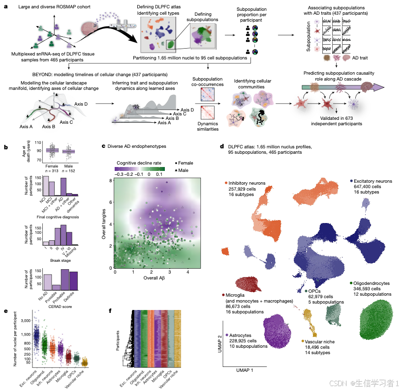
图2
source("5. Manuscript code/utils.R")
#####################################################################################################################
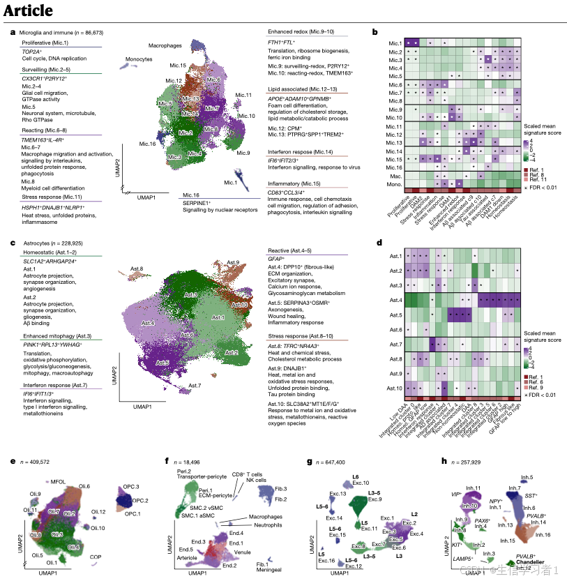
# Figure 2 - Cell-State Characterization #
#####################################################################################################################
# ----------------------------------------------------------------------------------------------------------------- #
# Cell-type UMAPS #
# ----------------------------------------------------------------------------------------------------------------- #
plot.umap <- function(name, cols=NULL) {
embedding <- h5read(aggregated.data, name)
st <- embedding$state %>% unique()
# If not specified randomly assign colors to states
if(is.null(cols)) {
cols <- unlist(lapply(split(1:length(st), 1:3), length))
cols <- setNames(c(colorRange("darkgreen")(cols[[1]]), colorRange("darkorchid4")(cols[[2]]), colorRange("midnightblue")(cols[[3]])), sample(st))
}
# Annotate plot with number of nuclei
text <- annotations[embedding$cell,] %>%
group_by(grouping.by) %>% summarise(n=n()) %>%
mutate(label=paste0(grouping.by," n=", n)) %>%
pull(label) %>% paste0(collapse = "\n")
pos <- apply(embedding[c("x","y")], 2, min)
return(ggplot(embedding, aes(x, y, color=state, label=state)) +
scale_color_manual(values=cols) +
ggrastr::geom_point_rast(size=.01, raster.dpi = 800) +
geom_text(data = embedding %>% group_by(state) %>% summarise_at(vars(x, y), list(mean)), color="black") +
annotate(geom = "text", label=text, x=pos[1], y=pos[2], hjust=0)+
no.labs +
theme_embedding +
theme(legend.position = "none"))
}
pdf(file.path(panel.path, "2.UMAPs.pdf"), width=embed.width, height = embed.height)
for(ct in c("vascular.niche","microglia","astrocytes","oligodendroglia","inhibitory","excitatory","neuronal")) {
plot.umap(file.path(mapping[[ct]], ifelse(ct %in% c("excitatory","neuronal"), "umap.ref","umap")),
cols = state.colors[[ct]]) %>% print(.)
}
while (!is.null(dev.list())) dev.off()
rm(ct, plot.umap)
# ----------------------------------------------------------------------------------------------------------------- #
# State QCs #
# ----------------------------------------------------------------------------------------------------------------- #
pdf(file.path(panel.path, "2.QCs.pdf"), width=embed.width, height=embed.height)
for(ct in names(atlas)) {
o <- LoadH5Seurat(paste0(ct,"/data/", ct, ".H5Seurat"), assays=list(SCT=c("data")), misc=F, graphs=F, reductions=F, neighbors=F, verbose=F)
Idents(o) <- factor(as.character(Idents(o)), levels=atlas[[ct]]$state.order)
if(any(is.na(Idents(o))))
o <- subset(o, cells = colnames(o)[!is.na(Idents(o))])
plot_grid(
VlnPlot(o, features=c("nCount_RNA","nFeature_RNA"), pt.size = 0, ncol = 1, log = TRUE, cols = state.colors[[ct]]) &
labs(x=NULL, y=NULL, title=NULL) &
NoLegend() &
theme(axis.text.x = element_blank()),
melt(data$X) %>%
`colnames<-`(c("donor","state","prev")) %>%
filter(state %in% levels(Idents(o))) %>%
mutate(state = factor(state, levels = levels(Idents(o)))) %>%
ggplot(aes(state, prev, fill=state, color=state)) +
geom_boxplot(alpha=.3, outlier.shape = NA) +
geom_jitter(size=.5, width=.2, alpha=.75) +
scale_color_manual(values=state.colors[[ct]]) +
scale_fill_manual(values=state.colors[[ct]]) +
scale_y_sqrt(breaks = c(.01, .05, .1, .25, .5, .75), labels = paste0(as.integer(100*c(.01, .05, .1, .25, .5, .75)), "%"), expand = expansion(0)) +
labs(x=NULL, y=NULL) +
theme_classic() +
theme(legend.position = "none"),
ncol=1,
rel_heights = c(1,1)) %>% print(.)
rm(o); gc()
}
while (!is.null(dev.list())) dev.off()
rm(ct)
# ----------------------------------------------------------------------------------------------------------------- #
# Signature scores #
# ----------------------------------------------------------------------------------------------------------------- #
# Removing Sadick et al annotations in favor of their integrated annotations
excluded.signatures = list(dummy=c("ABC"), `Sadick J.S. et al (2022)`=c())
pdf(file.path(panel.path, "2.signatures.pdf"), height=embed.height*1.25, width = embed.width*1.5)
for(ct in c("endo","microglia","astrocytes","oligodendroglia")) {
sigs <- h5read(aggregated.data, file.path(mapping[[ct]], "signatures"))
sigs$scores <- sigs$scores %>% mutate(sig.full=paste(reference, signature)) %>%
# Remove specified signatures
merge(., stack(excluded.signatures) %>% `colnames<-`(c("signature","reference")) %>% mutate(to.exclude=T), all.x=T) %>%
filter(is.na(to.exclude)) %>%
dplyr::select(-to.exclude) %>%
# Remove all signatures from specified references
filter(! reference %in% names(Filter(is.null, excluded.signatures)))
labels <- sigs$scores %>% dplyr::select(sig.full, signature) %>% unique %>% `rownames<-`(NULL) %>% column_to_rownames("sig.full")
references <- sigs$scores %>% dplyr::select(sig.full, reference) %>% unique %>% `rownames<-`(NULL) %>% column_to_rownames("sig.full")
mtx <- sigs$scores %>% pivot_wider(id_cols = "state", names_from = "sig.full", values_from = "mean") %>%
column_to_rownames("state") %>%
`[`(atlas[[ct]]$state.order, ) %>%
scale
significance <- sigs$scores %>%
rowwise() %>%
mutate(sig = ifelse(p.adjust <= .01, "*", "")) %>%
pivot_wider(id_cols = "state", names_from = "sig.full", values_from = "sig", values_fill = "") %>%
column_to_rownames("state") %>%
`[`(rownames(mtx), colnames(mtx)) %>%
as.matrix()
v <- max(abs(mtx), na.rm = T)
draw(Heatmap(mtx,
col = circlize::colorRamp2(seq(-v, v, length.out=21), green2purple(21)),
cluster_rows=F,
row_split = atlas[[ct]]$main.group,
show_column_dend = F,
column_labels = labels[colnames(mtx),],
column_names_rot = 45,
row_title = " ",
layer_fun = function(j, i, x, y, w, h, fill) grid.text(pindex(significance, i, j), x, y),
bottom_annotation = HeatmapAnnotation(ref=references[colnames(mtx),]),
height = unit(18, "cm"),
width = unit(14, "cm"),
border=T,
row_gap = unit(0,"pt")
), merge_legend=T)
}
while (!is.null(dev.list())) dev.off()
rm(ct, sigs, labels, references, mtx, significance, v,excluded.signatures)
# ----------------------------------------------------------------------------------------------------------------- #
# Signature gene expression #
# ----------------------------------------------------------------------------------------------------------------- #
# Removing Sadick et al annotations in favor of their integrated annotations
excluded.signatures = list(dummy=c("ABC"), `Sadick J.S. et al (2022)`=c())
pdf(file.path(panel.path, "2.signatures.genes.pdf"), height=embed.height*3, width = embed.width*1.5)
for(ct in c("vascular.niche","microglia","astrocytes","oligodendroglia")) {
# Load signatures' gene sets
sigs <- h5read(aggregated.data, file.path(mapping[[ct]], "signatures"))
sigs <- sigs$genes %>% mutate(section=paste(reference, signature), col=paste(reference, signature, gene)) %>%
# Remove specified signatures
merge(., stack(excluded.signatures) %>% `colnames<-`(c("signature","reference")) %>% mutate(to.exclude=T), all.x=T) %>%
filter(is.na(to.exclude)) %>%
dplyr::select(-to.exclude) %>%
# Remove all signatures from specified references
filter(! reference %in% names(Filter(is.null, excluded.signatures)))
de <- h5read(aggregated.data, file.path(mapping[[ct]], "de")) %>%
filter(avg_log2FC > 0 & p_val_adj < .01 & gene %in% unique(sigs$gene)) %>%
mutate(sig = "*") %>%
dplyr::select(cluster, gene, sig)
exp <- h5read(aggregated.data, file.path(mapping[[ct]], "gene.exp")) %>% filter(gene %in% unique(sigs$gene))
# Append expression levels and if gene is DE in state
df <- sigs %>%
merge(., exp, by.x = "gene", by.y="gene", all.x = T) %>%
merge(., de, by.x = c("state","gene"), by.y=c("cluster","gene"), all.x = T) %>%
mutate(sig = replace_na(sig, " "))
mtx <- pivot_wider(df %>% filter(!is.na(state)), id_cols = "state", names_from = "col", values_from = "mean.exp", values_fill = 0) %>%
column_to_rownames("state") %>%
`[`(atlas[[ct]]$state.order, intersect(sigs$col,colnames(.))) %>%
as.matrix %>%
scale %>%
t
significance <- pivot_wider(df %>% filter(!is.na(state)), id_cols = "state", names_from = "col", values_from = "sig", values_fill = "") %>%
column_to_rownames("state") %>%
`[`(atlas[[ct]]$state.order, intersect(sigs$col,colnames(.))) %>%
t
labeling <- sigs %>% column_to_rownames("col") %>% mutate(section = gsub(" .* ", " - ", section)) %>% `[`(intersect(sigs$col, rownames(mtx)),)
gaps <- labeling %>% dplyr::select(reference, section) %>% unique() %>% mutate(gap = ifelse(reference == lag(reference), 0, 3)) %>% pull(gap) %>% Filter(Negate(is.na), .)
draw(Heatmap(mtx,
col = green2purple(21),
cluster_columns = F,
column_labels = case_when(ct == "vascular.niche"~colnames(mtx), T~gsub("^.*\\.", "", colnames(mtx))),
column_names_rot = 0,
row_labels = labeling$gene,
row_split = labeling$section,
cluster_rows = T,
cluster_row_slices = F,
show_row_dend = F,
layer_fun = function(j, i, x, y, w, h, fill) grid.text(pindex(significance, i, j), x, y),
left_annotation = rowAnnotation(ref = labeling$reference),
heatmap_legend_param = list(title = "scaled mean exp."),
border=T,
row_gap = unit(gaps, "pt"),
width = unit(5,"cm"),
height= unit(20, "cm")))
}
while (!is.null(dev.list())) dev.off()
rm(ct, sigs, de, exp, df, mtx, significance, labeling)
# ----------------------------------------------------------------------------------------------------------------- #
# Dotplots of top and selected DEGs #
# ----------------------------------------------------------------------------------------------------------------- #
n.genes = list(inhibitory=4, excitatory=4, endo=4, astrocytes=3, oligodendroglia=4, microglia=3)
pdf(file.path(panel.path, "2.dotplots.pdf"), height=embed.height, width = embed.width*2)
for(ct in names(atlas)) {
additional.genes = c()
if("genes" %in% names(atlas[[ct]]))
additional.genes = unname(unlist(atlas[[ct]]$genes))
genes <- h5read(aggregated.data, file.path(mapping[[ct]], "de")) %>%
filter(avg_log2FC > 0) %>%
group_by(gene) %>%
slice_max(avg_log2FC, n=1) %>%
group_by(cluster) %>%
arrange(desc(avg_log2FC)) %>%
filter(row_number() <= n.genes[[ct]] | gene %in% additional.genes) %>%
unstack(gene~cluster) %>%
as.list
hm <- h5read(aggregated.data, file.path(mapping[[ct]], "gene.exp")) %>%
filter(gene %in% (genes[atlas[[ct]]$state.order] %>% unlist)) %>%
gheatmap(color.by="mean.exp", size.by="pct.exp",
row.order = list(a=atlas[[ct]]$state.order),
column.order = genes[atlas[[ct]]$state.order],
cluster_columns=FALSE, column_gap = unit(0, "mm"),
cols = green2purple,
border=TRUE,
cluster_rows=FALSE, scale="col")
draw(hm[[1]], merge_legend=TRUE, annotation_legend_list=hm[[2]])
}
while (!is.null(dev.list())) dev.off()
rm(ct, genes, hm, additional.genes, n.genes)
# ----------------------------------------------------------------------------------------------------------------- #
# Dotplots of top and selected DEGs - Oligodendroglia specific #
# ----------------------------------------------------------------------------------------------------------------- #
# Retrieve oligodendroglia DEGs + pseudobulk gene expression
de <- h5read(aggregated.data, file.path(mapping[["oligodendroglia"]], "de")) %>% filter(avg_log2FC > 0)
exp <- h5read(aggregated.data, file.path(mapping[["oligodendroglia"]], "gene.exp"))
# Create general OPC vs Oligo heatmap
genes <- list(OPCs=c("PCDH15", "VCAN", "PDGFRA"),
Oligodendrocytes=c("MBP", "MOG", "MAG"))
ct.hm <- exp %>% filter(gene %in% unlist(genes)) %>%
gheatmap(color.by="mean.exp", size.by="pct.exp",
name = "Cell-type marker",
row.order = list(a=atlas$oligodendroglia$state.order),
column.order = genes,
cluster_columns=FALSE, column_gap = unit(0, "mm"),
cols = green2purple,
border=TRUE,
cluster_rows=FALSE, scale="col")
# Create within OPCs and within Oligos heatmaps
states <- atlas$oligodendroglia$state.order %>% split(., if_else(grepl("Oli.", .),"Oligodendrocytes", "OPCs"))
additional.genes <- list(
OPCs = c("PINK1", "TOMM20", "TOMM7", "SERPINA3", "OSMR", "CNTN2", "SOX10", "SOX6"),
Oligodendrocytes = c("QDPR", "DPYD", "S100A6", "SEMA3C", "SLC38A2", "DNAJB1", "DNAJB6", "DNAJC1", "HSPA1A", "HSPA1B", "HSPA4L", "HSPH1", "PTGES3"))
hms <- lapply(names(states), \(ct) {
genes <- de %>%
filter(cluster %in% states[[ct]]) %>%
group_by(gene) %>%
slice_max(avg_log2FC, n=1) %>%
group_by(cluster) %>%
arrange(desc(avg_log2FC)) %>%
filter(row_number() <= 3 | gene %in% additional.genes[[ct]]) %>%
unstack(gene~cluster) %>% as.list
exp %>% filter(gene %in% unlist(genes)) %>%
gheatmap(color.by="mean.exp", size.by="pct.exp",
name = paste0(ct, "\nmean exp."),
row.order = list(a=atlas$oligodendroglia$state.order),
column.order = genes[states[[ct]]],
cluster_columns=FALSE, column_gap = unit(0, "mm"),
cols = green2purple,
border=TRUE,
cluster_rows=FALSE, scale="col")
})
pdf(file.path(panel.path, "2.dotplots.oligodendroglia.specific.pdf"), height=embed.height, width = embed.width*2)
draw(ct.hm[[1]] + hm[[2]][[1]] + hm[[1]][[1]] , merge_legend=TRUE,
annotation_legend_list=hm[[1]][[2]][[1]])
dev.off()
# ----------------------------------------------------------------------------------------------------------------- #
# Clustering-goodness confusion plots #
# ----------------------------------------------------------------------------------------------------------------- #
library(SeuratDisk)
library(dplyr)
library(Seurat)
objs <- c(sapply(c("microglia","astrocytes","oligodendroglia","inhibitory"),
\(ct) paste0(ct, "/data/", ct, ".h5Seurat")),
endo = "vascular.niche/data/vascular.niche.h5Seurat",
`cux2-`="excitatory/data/cux2-.h5Seurat",
`cux2+`="excitatory/data/cux2+.h5Seurat")
for (ct in names(objs)) {
message(ct)
obj <- LoadH5Seurat(objs[[ct]], assays=list(SCT=c("data")), verbose=F)
clusters <- Idents(obj)
if(! "SCT_snn" %in% names(obj@graphs))
obj <- FindNeighbors(obj, reduction="pca", dims = 1:50)
combs <- expand.grid(clusters %>% unique() %>% as.vector(),
clusters %>% unique() %>% as.vector()) %>% t()
dists <- apply(combs, 2, function(pair_){
cells1 <- names(clusters)[clusters == pair_[[1]] %>% as.vector()]
cells2 <- names(clusters)[clusters == pair_[[2]] %>% as.vector()]
(rowSums(obj@graphs$SCT_snn[cells1, cells2])/rowSums(obj@graphs$SCT_snn[cells1, ])) %>% mean()
})
saveRDS(list(dists = rbind(combs, dists) %>% t() %>% as.data.frame() %>% tidyr::spread(Var1, dists) %>% tibble::column_to_rownames("Var2"),
clusters = clusters), paste0("5. Manuscript code/data/", ct, ".knn.rds"))
rm(obj, clusters, combs, dists)
}
pdf(file.path(panel.path, "2.cluster.goodness.confusions.pdf"), height=embed.height*2, width = embed.width*2)
for(ct in names(objs)) {
df <- readRDS(paste0("5. Manuscript code/data/", ct, ".knn.rds"))
mtx <- sapply(df$dists, as.numeric) %>% `rownames<-`(rownames(df$dists))
if(ct %in% c("cux2+", "cux2-"))
ord <- intersect(atlas$excitatory$state.order, rownames(mtx))
else
ord <- atlas[[ct]]$state.order
Heatmap(t(mtx[ord, ord]),
width = unit(embed.width, "cm"), height = unit(embed.height, "cm"),
col=colorRampPalette(c("white","darkgreen","#5F9E5F","#A074B6","darkorchid4"))(21),
cluster_rows = F, cluster_columns = F, border=T) %>% draw()
}
while (!is.null(dev.list())) dev.off()
# ----------------------------------------------------------------------------------------------------------------- #
# Heatmaps of predicted neuronal subtypes #
# ----------------------------------------------------------------------------------------------------------------- #
neurons <- merge(annotations %>% rownames_to_column("cell"), h5read(aggregated.data, "neuronal/allen.annotations")) %>%
count(grouping.by, state, allen.labels) %>%
group_by(grouping.by, state) %>%
mutate(prop = n/sum(n)) %>%
ungroup()
neuronal.subtypes <- neurons %>%
select(allen.labels) %>% unique %>%
tidyr::separate(col = "allen.labels", sep = " ", into = c("type", "layer", "marker.1", "marker.2"), extra = "merge", remove = FALSE) %>%
mutate(marker.1 = factor(marker.1, rev(c("LAMP5", "PAX6", "SST", "VIP", "PVALB","RORB", "LINC00507","THEMIS","FEZF2"))),
across(c(layer, marker.2), ~factor(., sort(unique(.))))) %>%
column_to_rownames("allen.labels")
ord <- c(
"Exc L2 LINC00507 GLRA3", "Exc L2 LAMP5 KCNG3", "Exc L2 LINC00507 ATP7B", "Exc L2-3 LINC00507 DSG3",
"Exc L3 LAMP5 CARM1P1", "Exc L3 THEMIS ENPEP", "Exc L2-3 RORB RTKN2", "Exc L2-3 RORB PTPN3",
"Exc L2-3 RORB CCDC68", "Exc L3-5 RORB TNNT2", "Exc L3-5 RORB LAMA4", "Exc L3 RORB OTOGL",
"Exc L3-5 RORB LINC01202", "Exc L3-5 RORB LNX2", "Exc L3-5 RORB RPRM", "Exc L5 THEMIS SLC22A18",
"Exc L6 THEMIS LINC00343", "Exc L6 THEMIS SNTG2", "Exc L5-6 THEMIS TNFAIP6", "Exc L6 THEMIS SLN",
"Exc L5 RORB MED8", "Exc L5 THEMIS FGF10", "Exc L5 THEMIS VILL", "Exc L5-6 FEZF2 IFNG-AS1",
"Exc L5 FEZF2 NREP-AS1", "Exc L5 FEZF2 RNF144A-AS1", "Exc L5 FEZF2 PKD2L1", "Exc L5-6 FEZF2 LPO",
"Exc L6 FEZF2 KLK7", "Exc L6 FEZF2 POGK", "Exc L6 FEZF2 FFAR4", "Exc L6 FEZF2 PROKR2",
"Exc L5-6 FEZF2 CFTR", "Exc L6 FEZF2 PDYN", "Exc L5-6 FEZF2 C9orf135-AS1", "Exc L5-6 FEZF2 SH2D1B",
"Exc L5 THEMIS RGPD6", "Exc L5-6 FEZF2 FILIP1L", "Exc L5-6 FEZF2 OR1L8", "Exc L5 THEMIS LINC01116",
"Exc L5-6 THEMIS SMYD1", "Exc L5 FEZF2 CSN1S1", "Exc L3-5 FEZF2 ASGR2", "Exc L3-5 FEZF2 LINC01107",
"Inh L1-6 SST NPY", "Inh L1-6 LAMP5 AARD", "Inh L1 LAMP5 RAB11FIP1", "Inh L1-6 LAMP5 NES", "Inh L5-6 LAMP5 CRABP1",
"Inh L1-6 LAMP5 CA1", "Inh L1 PAX6 MIR101-1", "Inh L3-6 PAX6 LINC01497", "Inh L5-6 SST BEAN1",
"Inh L5-6 SST DNAJC14", "Inh L5-6 SST KLHL1", "Inh L5-6 SST FBN2", "Inh L5-6 SST C4orf26",
"Inh L1-2 SST PRRT4", "Inh L3-5 SST GGTLC3", "Inh L1-2 SST CLIC6", "Inh L2 PVALB FRZB",
"Inh L2-3 SST NMU", "Inh L1-2 SST CCNJL", "Inh L1-3 SST FAM20A", "Inh L3-5 SST CDH3",
"Inh L5 SST RPL35AP11", "Inh L5-6 SST PAWR", "Inh L3-5 SST OR5AH1P", "Inh L5-6 SST PIK3CD",
"Inh L5-6 PVALB SST CRHR2", "Inh L5-6 SST ISX", "Inh L1 SST DEFB108B", "Inh L1 LAMP5 BMP2",
"Inh L1 PVALB SST ASIC4", "Inh L1 PAX6 CHRFAM7A", "Inh L1-6 VIP SLC7A6OS", "Inh L1 LAMP5 PVRL2",
"Inh L1 SST P4HA3", "Inh L1 LAMP5 NMBR", "Inh L2 PAX6 FREM2", "Inh L1-2 VIP HTR3A", "Inh L1-2 VIP WNT4",
"Inh L1-5 VIP PHLDB3", "Inh L1-5 VIP LINC01013", "Inh L3-6 VIP UG0898H09", "Inh L3-6 VIP ZIM2-AS1",
"Inh L1-5 VIP CD27-AS1", "Inh L2-5 VIP SOX11", "Inh L1-2 VIP PTGER3", "Inh L2-5 VIP BSPRY", "Inh L5-6 VIP COL4A3",
"Inh L1-2 VIP SCML4", "Inh L2 VIP SLC6A16", "Inh L1-3 VIP HSPB6", "Inh L1-5 VIP SMOC1", "Inh L1-3 VIP CHRNA2",
"Inh L3-5 VIP HS3ST3A1", "Inh L1-2 VIP EXPH5", "Inh L1-3 VIP FNDC1", "Inh L1 VIP KLHDC8B", "Inh L1-3 VIP CBLN1",
"Inh L3-5 VIP IGDCC3", "Inh L3-5 VIP TAC3", "Inh L1-6 PVALB COL15A1", "Inh L5-6 PVALB ZFPM2-AS1",
"Inh L6 SST TH", "Inh L5-6 PVALB GAPDHP60", "Inh L5-6 PVALB KCNIP2", "Inh L1-2 SST CLIC6",
"Inh L2 PVALB FRZB", "Inh L2-5 PVALB RPH3AL", "Inh L1-2 PVALB CDK20", "Inh L3 PVALB SAMD13",
"Inh L3-5 PVALB ISG20", "Inh L2-5 PVALB HHIPL1", "Inh L5-6 PVALB FAM150B", "Inh L5-6 PVALB MEPE", "Inh L5 PVALB LRIG3")
sets = list(c("Inhibitory Neurons", "inhibitory"), c("Excitatory Neurons", "excitatory"))
pdf(file.path(panel.path, "2.neuronal.confusions.pdf"), height=embed.height*2, width = embed.width*2)
for(set in sets) {
df <- pivot_wider(neurons %>% filter(grouping.by == set[[1]]), id_cols="allen.labels", names_from = "state", values_from = "prop", values_fill = 0) %>%
column_to_rownames("allen.labels") %>%
`[`(intersect(v, rownames(.)), atlas[[set[[2]]]]$state.order) %>%
as.matrix
Heatmap(df,
col=colorRampPalette(c("white","darkgreen","#5F9E5F","#A074B6","darkorchid4"))(21),
width = unit(ncol(df)*.35,"cm"),
border=T,
column_order = atlas[[set[[2]]]]$state.order,
cluster_rows = F, cluster_row_slices = F,
right_annotation = rowAnnotation(
`Cortical layer` = anno_text(paste(neuronal.subtypes[rownames(df), "layer"], " ")),
`Marker 1` = anno_text(paste(neuronal.subtypes[rownames(df), "marker.1"], " ")),
`Marker 2` = anno_text(neuronal.subtypes[rownames(df), "marker.2"])
),
left_annotation = rowAnnotation(
`Cortical layer` = neuronal.subtypes[rownames(df), "layer"],
marker1 = neuronal.subtypes[rownames(df), "marker.1"]),
show_row_names = F) %>% draw()
}
while (!is.null(dev.list())) dev.off()
rm(df, sets, set, ord, neuronal.subtypes, neurons)
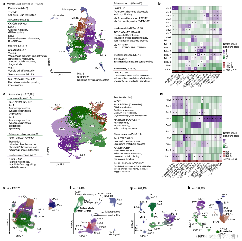
图3
source("5. Manuscript code/utils.R")


#####################################################################################################################
#                                    Figure 3 - State-Trait Associations & Validations                              #
#####################################################################################################################

# ----------------------------------------------------------------------------------------------------------------- #
#                                  Panel B+C - joint - snuc+bulk Trait Associations                                 #
# ----------------------------------------------------------------------------------------------------------------- #

pdf(file.path(panel.path, "3B-D.pdf"), width=2*3 + 1, height=5)
plot.trait.associations.cross.cohort(
  names(AD.traits), AD.traits, fdr.thr = .01, use_raster=TRUE, raster_quality = 10)
while (!is.null(dev.list()))  dev.off()


# ----------------------------------------------------------------------------------------------------------------- #
#                                     Panel B+C - snuc+bulk Trait Associations                                      #
# ----------------------------------------------------------------------------------------------------------------- #
pdf(file.path(panel.path, "3B.pdf"), width=3.5, height=5)
plot.trait.associations(py_to_r(data$uns$trait.analysis$snuc),
                        params = names(AD.traits),
                        column_title="snRNA-seq",
                        column_labels = AD.traits,
                        column_names_rot = 45,
                        column_names_centered = T,
                        row_names_side = "left",
                        use_raster=T,
                        raster_quality = 10) %>% print()
while (!is.null(dev.list()))  dev.off()


pdf(file.path(panel.path, "3C.pdf"), width=3.5, height=5)
plot.trait.associations(py_to_r(data$uns$trait.analysis$celmod),
                        params = names(AD.traits),
                        column_title="bulk-predicted",
                        column_labels = AD.traits,
                        column_names_rot = 45,
                        column_names_centered = T,
                        row_names_side = "left",
                        use_raster=T,
                        raster_quality = 10) %>% print()
while (!is.null(dev.list()))  dev.off()


# ----------------------------------------------------------------------------------------------------------------- #
#                                      Panel D - Meta analysis of associations                                      #
# ----------------------------------------------------------------------------------------------------------------- #
pdf(file.path(panel.path, "3D.pdf"), width=3.5, height=5)
plot.trait.associations(py_to_r(data$uns$trait.analysis$meta.analysis),
                        params = names(AD.traits),
                        value.by = "z.meta", pval.by = "adj.pval.meta",
                        column_title="meta-analysis",
                        column_labels = AD.traits,
                        column_names_rot = 45,
                        column_names_centered = T,
                        row_names_side = "left") %>% print()
while (!is.null(dev.list()))  dev.off()


# ----------------------------------------------------------------------------------------------------------------- #
#                                             Panels F-J - Causal modeling                                          #
# ----------------------------------------------------------------------------------------------------------------- #
# Panels were designed based on the results in the Other analyses/3.causal modeling.R file


#####################################################################################################################
#                                 Supp Figure 3 - State-Trait Associations & Validations                            #
#####################################################################################################################


# ----------------------------------------------------------------------------------------------------------------- #
#                                         Panel A - CelMod correlations for states                                  #
# ----------------------------------------------------------------------------------------------------------------- #
pdf(file.path(panel.path, "s6A.pdf"), width=14, height=3)
print(py_to_r(data$uns$celmod$test.corrs) %>%
        rownames_to_column("state") %>%
        mutate(group = factor(data$var[state, "grouping.by"], levels=names(cell.group.color))) %>%
        ggplot(aes(reorder(state, -corr),corr, fill=group, label=sig)) +
        geom_bar(stat="identity") +
        geom_text(nudge_y = .01, angle=90, hjust=0, vjust=.65) +
        facet_wrap(.~group, scales = "free_x", nrow = 1) +
        scale_fill_manual(values=scales::alpha(cell.group.color, .75)) +
        scale_y_continuous(expand = expansion(add=c(.1, .2))) +
        labs(x=NULL, y=NULL) +
        theme_classic() +
        theme(legend.position = "none",
              strip.background = element_blank(),
              axis.text.x = element_text(angle=90, hjust = 1, vjust = .5)))
while (!is.null(dev.list()))  dev.off()


# ----------------------------------------------------------------------------------------------------------------- #
#                                       Panel B - snRNAseq/bulk tstat comparison                                   #
# ----------------------------------------------------------------------------------------------------------------- #

pdf(file.path(panel.path, "s6B.pdf"), width=embed.width, height=embed.height.small*3)
traits = c(AD.traits, AD.traits.cat)
  df <- py_to_r(data$uns$trait.analysis$meta.analysis) %>%
    filter(trait %in% names(traits)) %>%
    group_by(trait) %>%
    mutate(trait = factor(trait, names(traits)),
           label = if_else(adj.pval.meta <= .05, state, NA_character_),
           color = case_when(is.na(label) ~ NA_character_,
                             tstat.sc > 0 ~ "1",
                             tstat.sc < 0 ~ "-1"))


  corrs <- do.call(rbind, lapply(unique(df$trait), function(t)
    data.frame(cor.test(df[df$trait == t,]$tstat.sc,
                        df[df$trait == t, ]$tstat.b,
                        method="spearman")[c("estimate","p.value")], row.names = t))) %>%
    mutate(adj.pval = p.adjust(p.value, method = "BH"))


  plot_grid(plotlist = lapply(levels(df$trait), function(t) {
    .df <- df[df$trait == t,]

    range.min <- min(.df[,c("tstat.sc","tstat.b")], na.rm = T)
    range.max <- max(.df[,c("tstat.sc","tstat.b")], na.rm = T)

    .label <- paste0("R=", round(corrs[t,]$estimate, 2),
                     "\nFDR=", scales::scientific(corrs[t,]$adj.pval))

    ggplot(.df, aes(tstat.sc, tstat.b, label=label)) +
      geom_abline(linetype="dashed", color="grey30") +
      geom_point(size=.75) +
      ggplot2::annotate(geom="text", x=range.min, y=.95*range.max, hjust=0, vjust=1,label=.label) +
      ggrepel::geom_text_repel(aes(color=color), max.overlaps = 30, show.legend = F, min.segment.length = unit(0, "pt")) +
      scale_color_manual(values = list("1"=green2purple(3)[3], "-1"=green2purple(3)[1])) +
      scale_x_continuous(limits = c(range.min, range.max), expand = expansion(mult = .025)) +
      scale_y_continuous(limits = c(range.min, range.max), expand = expansion(mult = .025)) +
      labs(x="t-stat snRNA-seq", y="t-stat bulk pred.", title=traits[[t]])
  }),
  nrow=3) %>% print()
rm(df, corrs, traits)
while (!is.null(dev.list()))  dev.off()


# ----------------------------------------------------------------------------------------------------------------- #
#                                       Panel C - snuc+bulk Trait Associations                                      #
# ----------------------------------------------------------------------------------------------------------------- #

pdf(file.path(panel.path, "s6C.joint.pdf"), width=2*3 + 1, height=5)
plot.trait.associations.cross.cohort(names(AD.traits.cat), AD.traits.cat,
                                     fdr.thr = .01, use_raster=TRUE, raster_quality = 10)
while (!is.null(dev.list()))  dev.off()


pdf(file.path(panel.path, "s6C.pdf"), width=3.5, height=5)
plot.trait.associations(py_to_r(data$uns$trait.analysis$snuc),
                        params = names(AD.traits.cat),
                        column_title="snRNA-seq",
                        column_labels = AD.traits.cat,
                        column_names_rot = 45,
                        column_names_centered = T,
                        row_names_side = "left",
                        use_raster=T,
                        raster_quality = 10) %>% print()

plot.trait.associations(py_to_r(data$uns$trait.analysis$celmod),
                        params = names(AD.traits.cat),
                        column_title="bulk-predicted",
                        column_labels = AD.traits.cat,
                        column_names_rot = 45,
                        column_names_centered = T,
                        row_names_side = "left",
                        use_raster=T,
                        raster_quality = 10) %>% print()

plot.trait.associations(py_to_r(data$uns$trait.analysis$meta.analysis),
                        params = names(AD.traits.cat),
                        value.by = "z.meta", pval.by = "adj.pval.meta",
                        column_title="meta-analysis",
                        column_labels = AD.traits.cat,
                        column_names_rot = 45,
                        column_names_centered = T,
                        row_names_side = "left") %>% print()
while (!is.null(dev.list()))  dev.off()


# ----------------------------------------------------------------------------------------------------------------- #
#                                             Panels D-I - Causal modeling                                          #
# ----------------------------------------------------------------------------------------------------------------- #
# Panels were designed based on the results in the `3. Other analyses/3.causal modeling.R` file
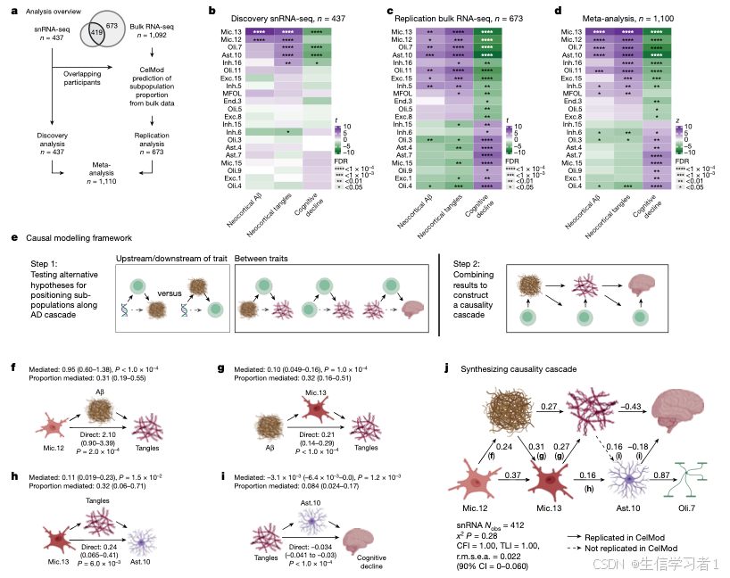
图4
source("5. Manuscript code/utils.R")

# The following results file is generated by `Other analyses/RNAscope.analysis.R`
validations <- readRDS("3. Other analyses/data/RNAscope.rds")

#####################################################################################################################
#                                           Figure 4 - RNAscope Validations                                         #
#####################################################################################################################


# ----------------------------------------------------------------------------------------------------------------- #
#                                           Panel A - Mic12/13 pathways vs all                                      #
# ----------------------------------------------------------------------------------------------------------------- #
pathways <- h5read(aggregated.data, file.path(mapping[["microglia"]], "pa")) %>%
  filter(state %in% c("Mic.12","Mic.13") & Count > 2) %>%
  mutate(direction.n = if_else(direction == "upregulated", 1, -1),
         signed.pval = -log10(p.adjust) * direction.n) %>%
  pivot_wider(id_cols = c("Description"), names_from = c(state, state), values_from = c(signed.pval, direction.n)) %>%
  mutate(across(contains("direction.n"), ~replace_na(., 0)),
         tot.direction = direction.n_Mic.12 + direction.n_Mic.13) %>%
  arrange(tot.direction, signed.pval_Mic.12, signed.pval_Mic.13) %>%
  column_to_rownames("Description")

annotate <- c("negative regulation of cell migration",
              "negative regulation of response to oxidative stress",
              "actin binding", "regulation of lipase activity",
              "foam cell differentiation", "lipid catabolic process",
              "lipid catabolic process", "exploration behavior",
              "glial cell migration", "synapse organization",
              "positive regulation of protein polymerization",
              "Platelet activation, signaling and aggregation")
annotate <- which(rownames(pathways) %in% annotate)

pdf(file.path(panel.path, "4A.pdf"), width=embed.width*.7, height=embed.height*1.2)
Heatmap(pathways %>% select(contains("signed.pval")) %>% as.matrix,
        col = green2purple.less.white(21),
        cluster_rows = F,
        cluster_columns = F,
        show_row_names = F,
        row_split = pathways$tot.direction,
        column_labels = c("Mic.12", "Mic.13"),
        row_title = " ",
        right_annotation = rowAnnotation(text=anno_mark(at=annotate, labels=rownames(pathways)[annotate])),
        border=T,
        row_gap = unit(0,"pt"),
        na_col = "grey90",
        height = unit(6,"cm"),
        width = unit(.8, "cm"))
while (!is.null(dev.list()))  dev.off()
rm(pathways, annotate)


# ----------------------------------------------------------------------------------------------------------------- #
#                                           Panel B - Mic12 vs Mic13 pathways                                       #
# ----------------------------------------------------------------------------------------------------------------- #
pathways <- h5read(aggregated.data, file.path(mapping[["microglia"]], "pa.pairwise")) %>%
  filter(comparison %in% c("Mic.12 vs. Mic.13","Mic.13 vs. Mic.12")) %>%
  dplyr::rename(state=comparison) %>%
  mutate(direction = ifelse(state == "Mic.13 vs. Mic.12", 1, -1), rowname=Description,
         signed.pval = -log10(p.adjust)*direction) %>%
  arrange(signed.pval) %>%
  column_to_rownames("rowname")


annotate = c("MHC class II protein complex", "negative regulation of leukocyte apoptotic process",
             "Antigen processing and presentation", "axonogenesis",
             "extracellular matrix organization", "cell junction assembly", "lamellipodium assembly",
             "lamellipodium assembly and organization", "negative regulation of immune system process",
             "negative regulation of locomotion", "immunological synapse")
annotate <- which(rownames(pathways) %in% annotate)

pdf(file.path(panel.path, "4B.pdf"), width=embed.width*.7, height=embed.height*1.2)
Heatmap(pathways %>% select(signed.pval) %>% as.matrix,
        col = green2purple(21),
        cluster_rows = F, show_row_names = F, show_column_names = F,
        row_title = " ",
        right_annotation = rowAnnotation(text=anno_mark(at=annotate, labels=rownames(pathways)[annotate])),
        row_split = pathways$direction,
        border=T,
        row_gap = unit(0,"pt"),
        height = unit(6,"cm"),
        width = unit(.4, "cm"))
while (!is.null(dev.list()))  dev.off()
rm(annotate, pathways)


# ----------------------------------------------------------------------------------------------------------------- #
#                                   Panel C - Selective genes differential between Mic12/13/Mac                     #
# ----------------------------------------------------------------------------------------------------------------- #

genes = list(`Mic.12 genes` = c("CD163","HLA-DRA","FOXP1","PELI1","PELI2"),
             `Both`         = c("MSR1","PRKCE"),
             `Mic.13 genes` = c("PTPRG","PPARG","SPP1","TGFBR1","SMAD3","SCIN","WIPF3"),
             `AD risk genes`= c("ADAM10","TREM2","APOE","GPNMB"))

exp <- h5read(aggregated.data, "glia/microglia/gene.exp") %>% filter(gene %in% unlist(genes))

# Summarize "other" microglia (non Mic.12/13/Mac/Mono) gene expression
n.mic <- exp %>% select(state, n) %>% unique %>% pull(n) %>% sum

exp <- exp %>% mutate(collapse.state = !state %in% c("Mic.12","Mic.13","Monocytes","Macrophages"),
                      state.prop = if_else(collapse.state, n/n.mic, 1),
                      state = if_else(collapse.state, "Other", state)) %>%
  mutate(mean.exp = mean.exp*state.prop,
         pct.exp = pct.exp*state.prop) %>%
  group_by(state, gene) %>%
  summarise(across(c(mean.exp, pct.exp), sum))


hm <- gheatmap(df = exp, color.by = "mean.exp", size.by="pct.exp", cols = green2purple,
           row.order = list(a=c("Monocytes","Macrophages","Mic.12","Mic.13","Other")), column.order = genes, scale.by = "col", cluster_rows=F, border=T, show_column_dend=F, cluster_columns=F)

pdf(file.path(panel.path, "4C.pdf"), width=10, height=3)
draw(hm[[1]], annotation_legend_list = hm[[2]], merge_legend=T)
while (!is.null(dev.list()))  dev.off()

rm(n.mic, exp, genes, hm)


# ----------------------------------------------------------------------------------------------------------------- #
#                                      Panel E - Markers Distributions - snRNAseq                                   #
# ----------------------------------------------------------------------------------------------------------------- #
# The following code produces scatter plots shown in panel 4e, as well as in Extended Data Figure 7d

cols <- c("Mic.12"="paleturquoise3", "Mic.13"="red3","Macrophages"="orchid3")

pdf(file.path(panel.path, "4E.pdf"), width=embed.width.small*3, height=embed.height.small*2)
ord <- list(c("TPRG1","CPM"), c("TPRG1","MRC1"), c("CPM","MRC1"))

snuc <- lapply(ord, function(pair)
  validations$RNAscope$snuc.exp %>%
    filter(state != "Other") %>%
    dplyr::select(state, g1=pair[[1]], g2=pair[[2]]) %>%
    mutate(group = factor(paste(pair, collapse = "-")),
           state = factor(state, levels = rev(c("Mic.12","Mic.13","Macrophages"))))) %>%
  do.call(rbind, .) %>%
  rowwise() %>%
  count(state, g1, g2, group) %>%
  `[`(sample(rownames(.)),) %>%
  ggplot(., aes(g1,g2, color=state)) +
  geom_jitter(alpha=.75) +
  scale_color_manual(values = cols) +
  scale_x_continuous(expand = expansion(add=2)) +
  scale_y_continuous(expand = expansion(add=2)) +
  facet_wrap("group", scales = "free") +
  labs(x=NULL, y=NULL, color=NULL) +
  guides(colour = guide_legend(override.aes = list(size=3)))  +
  theme_classic() +
  theme(strip.background = element_blank())

df <- validations$RNAscope$df %>%
  rowwise() %>%
  mutate(state = c("Mic.12","Mic.13","Macrophages", "Other", "none")[which.max(c_across(c(Mic.12,Mic.13,Macrophages, Other, none)))]) %>%
  data.frame

scope <- lapply(ord, function(pair) df %>% dplyr::select(state, g1=pair[[1]], g2=pair[[2]]) %>%
                  mutate(group = factor(paste(pair, collapse = "-")))) %>%
  do.call(rbind, .) %>%
  rowwise() %>%
  count(state, g1, g2, group) %>%
  mutate(state = factor(state, c("Mic.12","Mic.13","Macrophages"))) %>%
  `[`(sample(rownames(.)),) %>%
  ggplot(., aes(g1,g2, color=state)) +
  scale_alpha_binned(range=c(.1, .5))+
  geom_jitter(alpha=.75) +
  scale_x_continuous(expand = expansion(add=.2)) +
  scale_y_continuous(expand = expansion(add=.2)) +
  scale_color_manual(values = cols, na.value = "lightgrey") +
  guides(colour = guide_legend(override.aes = list(size=3)))  +
  facet_wrap("group", scales = "free") +
  labs(x=NULL, y=NULL) +
  theme_classic() +
  theme(strip.background = element_blank())

print(snuc / scope)
while (!is.null(dev.list()))  dev.off()
rm(snuc, scope, ord, df)


# ----------------------------------------------------------------------------------------------------------------- #
#                                        Panel F - Prevalence disease regression                                    #
# ----------------------------------------------------------------------------------------------------------------- #

pdf(file.path(panel.path, "4F.pdf"), width=embed.width.small, height=embed.height)
cols <- c("AD"="red3", "MCI"="chocolate2", "No AD"="#191970")
format <- paste(rep("t=%.2g, P=%.2g", 2), sep="*\", \"*")

merge(validations$RNAscope$predicted.proportions,
      validations$pTau$summarised,
      by.x = c("row.names","batch","AD"), by.y = c("sample","batch","AD")) %>%
  pivot_longer(cols = c(Mic.12,Mic.13), names_to = "state", values_to = "prop") %>%
  ggplot(aes(pTau_tangles_plaques_median, prop)) +
  geom_smooth(formula = "y~x", method="lm",color="black", alpha=.2) +
  ggpmisc::stat_fit_tidy(aes(label=sprintf(format, after_stat(`x_stat`), after_stat(`x_p.value`)))) +
  geom_point(aes(color=AD), size=2) +
  scale_color_manual(values = cols) +
  scale_y_continuous(expand = expansion(mult=.02), oob=scales::squish) +
  scale_x_continuous(expand = expansion(mult=.01)) +
  facet_wrap(~state, ncol=1, scales = "free") +
  labs(x=NULL, y=NULL) +
  theme_classic()  +
  theme(strip.background = element_blank(),
        legend.position = c(3,3))

rm(format, cols)
while (!is.null(dev.list()))  dev.off()


# ----------------------------------------------------------------------------------------------------------------- #
#                                        Panel G - associating morphology with state probability                    #
# ----------------------------------------------------------------------------------------------------------------- #

pdf(file.path(panel.path, "4G.pdf"), width=embed.width, height=embed.height)
split(validations$RNAscope$morpholoy.association, validations$RNAscope$morpholoy.association$trait) %>%
  lapply(., function(df) {
    v = max(abs(df$tstat))
    text = paste(round(df$tstat, 2), df$sig, sep = "\n")

    col.range <- green2purple(21)
    if(df[1,"trait"] == "eccentricity")
      col.range <- rev(col.range)

    Heatmap(df[,"tstat"],
            row_labels = df$state,
            cluster_rows = F,
            show_column_names = F,
            cluster_columns = F,
            width = unit(.8,"cm"),
            height = unit(8, "cm"),
            col = circlize::colorRamp2(seq(-v, v, length.out=21), col.range),
            cell_fun = function(j, i, x, y, w, h, col) grid.text(text[i], x,y),
            column_title = df[1,"trait"],
            row_names_side = "left",
            border=T,

            heatmap_legend_param = list(direction="horizontal", title="t stat"))
  }) %>% base::Reduce(`+`,.)
while (!is.null(dev.list()))  dev.off()


# ----------------------------------------------------------------------------------------------------------------- #
#                                             Panel H - PAM score for microglial states                             #
# ----------------------------------------------------------------------------------------------------------------- #
res <- validations$ROSMAP.PAM.Association
v   <- max(abs(res$t.value))

pdf(file.path(panel.path, "4H.pdf"), width=embed.width, height=embed.height)
plot_grid(
  Heatmap(res[1:4,"t.value"] %>% as.matrix(),
          col = circlize::colorRamp2(seq(-v, v, length.out=7), green2purple(7)),
          row_labels = rownames(res)[1:4],
          cluster_rows = F,
          show_column_names = F,
          row_names_side = "left",
          border=T,
          width = unit(.8,"cm"),
          height = unit(8,"cm"),
          column_title="PAM Score",
          heatmap_legend_param = list(title="t stat"),
          cell_fun = function(j, i, x, y, w, h, col) grid.text(paste(round(res[i, "t.value"],2), res[i, "sig"], sep = "\n"), x, y)) %>% draw %>% grid.grabExpr(),

  Heatmap(res[5:6,"t.value"] %>% as.matrix(),
          col = circlize::colorRamp2(seq(-v, v, length.out=7), green2purple(7)),
          cluster_rows = F,
          show_column_names = F,
          row_names_side = "left",
          border=T,
          width = unit(.8,"cm"),
          height = unit(4, "cm"),
          heatmap_legend_param = list(title="t stat"),
          cell_fun = function(j, i, x, y, w, h, col) grid.text(paste(round(res[i+4, "t.value"],2), res[i+4, "sig"], sep = "\n"), x, y)) %>% draw %>% grid.grabExpr(),
  align = "hv") %>% print(.)
while (!is.null(dev.list()))  dev.off()
rm(others, df, res, v, res.ctrl, controls)


# ----------------------------------------------------------------------------------------------------------------- #
#                                        Panel H - PAM scores with controls for confounders                         #
# ----------------------------------------------------------------------------------------------------------------- #
controls <- c("pmi", "Mic.12", "Mic.13")

pdf(file.path(panel.path, "4H.2.pdf"), width=embed.width, height=embed.height*2)
lapply(c("Mic.12","Mic.13"), function(state) {
  .df <- df %>% mutate(covariate = get(state))
  naive <- lm(pam ~ covariate, .df)

  # Controlling for confounding effects
  confounders <- lm(paste0("pam~", paste(setdiff(controls, state), collapse = "+")), .df)

  # Fitting pam to state after controlling for confounders
  fit <- lm(resid.pam ~ covariate, .df %>% mutate(resid.pam=residuals(confounders) + mean(.df$pam)))

  .df <- purrr::map2(list(naive, fit), c("direct", "controlled"),
                     ~predict(.x, se=T) %>% `[`(c("fit","se.fit")) %>% as.data.frame %>%
                       mutate(model=.y, state=state) %>% cbind(., .df[, c("pam","covariate")])) %>%
    do.call(rbind, .)

  ggplot(.df, aes(covariate, pam, group=model, fill=model, color=model)) +
    geom_ribbon(aes(ymin=fit-se.fit, ymax=fit+se.fit), alpha=.1, color=NA) +
    geom_line(aes(y=fit)) +
    geom_point(data=. %>% filter(model == "direct"), color="black") +
    labs(x=state, y="pam score")
}) %>% ggpubr::ggarrange(plotlist = ., ncol = 1, common.legend = T, legend="bottom")
while (!is.null(dev.list()))  dev.off()
rm(controls)


#####################################################################################################################
#                                       Supp Figure 4 - RNAscope Validations                                        #
#####################################################################################################################

# ----------------------------------------------------------------------------------------------------------------- #
#                              Panel A - Expression of key Mic.12/13 genes without collapsing states                #
# ----------------------------------------------------------------------------------------------------------------- #
genes = list(`Mic.12 genes` = c("CD163","HLA-DRA","FOXP1","PELI1","PELI2"),
             `Both`         = c("MSR1","PRKCE"),
             `Mic.13 genes` = c("PTPRG","PPARG","SPP1","TGFBR1","SMAD3","SCIN","WIPF3"),
             `AD risk genes`= c("ADAM10","TREM2","APOE","GPNMB"))
hm <- h5read(aggregated.data, "glia/microglia/gene.exp") %>%
  filter(gene %in% unlist(genes)) %>%
  gheatmap(color.by = "mean.exp", size.by="pct.exp", cols = green2purple,
           row.order = list(a=atlas$microglia$state.order), column.order = list(a=unlist(genes)), scale.by = "col", cluster_rows=F, border=T, show_column_dend=F, cluster_columns=F)

pdf(file.path(panel.path, "s7A.pdf"), width=7.5, height=5)
draw(hm[[1]], annotation_legend_list = hm[[2]], merge_legend=T)
while (!is.null(dev.list()))  dev.off()

rm(genes, hm)


# ----------------------------------------------------------------------------------------------------------------- #
#                                     Panel B - Expression of validation markers                                    #
# ----------------------------------------------------------------------------------------------------------------- #
res <- h5read(aggregated.data, file.path(mapping[["microglia"]], "gene.exp")) %>%
  filter(gene %in% c("CPM","TPRG1", "MRC1")) %>%
  mutate(pct.exp = 100*pct.exp) %>%
  gheatmap("state", "gene", "mean.exp", "pct.exp",
           scale.by = "col",
           cols = green2purple,
           cluster_columns = F,
           row_order = atlas$microglia$state.order,
           column_order = c("CPM","TPRG1", "MRC1"),
           row_names_side="left",
           cluster_rows=F,
           row_title = " ",
           border=T,
           size.by.round=0)

pdf(file.path(panel.path, "s7B.pdf"), width=embed.width*.75, height=embed.height)
draw(res[[1]], merge_legends=T, annotation_legend_list = res[[2]])
while (!is.null(dev.list()))  dev.off()
rm(res)
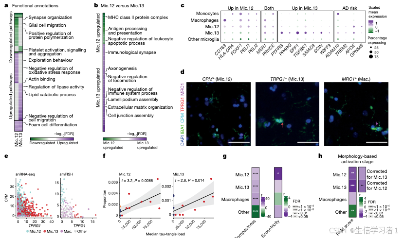
图5
source("5. Manuscript code/utils.R")


#####################################################################################################################
#                                  Figure 5 - Cellular Landscape & State/Trait Dynamics                             #
#####################################################################################################################


# ----------------------------------------------------------------------------------------------------------------- #
#                                            Panel B - Branch Probabilities                                         #
# ----------------------------------------------------------------------------------------------------------------- #
pdf(file.path(panel.path, "5B.pdf"), width=embed.width.small*.65, height=embed.height.small)
plot.landscape(data$uns$trajectories$palantir$branch.probs %>% py_to_r %>% mutate(diff=prAD-ABA) %>% dplyr::select(diff),
               smoothened = F,
               size = 1,
               cols = green2purple.less.white,
               legend.position = c(3,3))
while (!is.null(dev.list()))  dev.off()


# ----------------------------------------------------------------------------------------------------------------- #
#                                           Panel C - State Prevalence PHATE                                        #
# ----------------------------------------------------------------------------------------------------------------- #
pdf(file.path(panel.path, "5C.pdf"), width=embed.width.small*.75*4, height=embed.height.small*2)
plot.landscape(c("Ast.1", "Mic.12","Ast.10","Ast.5", "Mic.2","Mic.13","Oli.7","OPC.3"), enforce.same.color.scale = FALSE, smoothened = TRUE, ncol=4) %>% print(.)
while (!is.null(dev.list()))  dev.off()


# ----------------------------------------------------------------------------------------------------------------- #
#                                           Panel D - Trait Prevalence PHATE                                        #
# ----------------------------------------------------------------------------------------------------------------- #
pdf(file.path(panel.path, "5D.pdf"), width=embed.width.small*.75, height=embed.height.small*3)
plot_grid(
  plot.landscape(c("sqrt.amyloid_mf","sqrt.tangles_mf"), enforce.same.color.scale = FALSE, ncol = 1),
  plot.landscape(c("cogng_demog_slope"), cols = function(n) colorRampPalette(rev(c("#30123BFF", "#4777EFFF", "#1BD0D5FF", "#62FC6BFF", "#D2E935FF", "#FE9B2DFF", "#DB3A07FF")))(n), sort.direction = -1, enforce.same.color.scale = FALSE, ncol = 1),
  ncol=1, rel_heights = c(2,1)
)
while (!is.null(dev.list()))  dev.off()


# ----------------------------------------------------------------------------------------------------------------- #
#                                              Panel E - Trait Dynamics                                             #
# ----------------------------------------------------------------------------------------------------------------- #
pdf(file.path(panel.path, "5E.pdf"), width=embed.width, height=embed.height*1.75)
plot_grid(plotlist = lapply(names(AD.traits), function(trait)
  plot.dynamics(c(trait), dynamics = data$uns$trajectories$palantir$dynamics, cols=AD.traits.colors,
                overlap.pseudotime=.112, ncol=2, strip.position="top", scales="free",
                label = F, legend.position = c(2.5,0), include.points=F) +
    labs(x=NULL, y=trait, title=NULL)),
  ncol=1) %>% print()
while (!is.null(dev.list()))  dev.off()


# ----------------------------------------------------------------------------------------------------------------- #
#                                              Panel F - Landscape Bulk                                             #
# ----------------------------------------------------------------------------------------------------------------- #
bulk <- anndata::read_h5ad("4. BEYOND/data/Celmod.subpopulation.proportion.h5ad")

# prAD-ABA landscape
pdf(file.path(panel.path, "5F.traj.prob.pdf"), width=embed.width.small, height=embed.height.small)
plot.landscape(bulk$uns$trajectories$branch.probs %>% py_to_r %>% mutate(diff=prAD.like-ABA.like) %>% dplyr::select(diff),
               "X_umap",
               smoothened = F,
               size = 1,
               cols = green2purple.less.white,
               legend.position = c(3,3), data. = bulk)
while (!is.null(dev.list()))  dev.off()

# Trajectories root point
pdf(file.path(panel.path, "5F.root.pdf"), width=embed.width.small, height=embed.height.small)
plot.landscape(data$obs %>% mutate(root = if_else(data$uns$trajectories$pseudotime ==0, "root", NA_character_)) %>%
                 dplyr::select(root), "X_umap",data. = bulk)
while (!is.null(dev.list()))  dev.off()


# Landscape of key states
pdf(file.path(panel.path, "5F.states.pdf"), width=embed.width.small, height=embed.height.small)
plot.landscape(c("Ast.1","Ast.5","Ast.10","Mic.13"), "X_umap", enforce.same.color.scale = FALSE, size = 1, data. = bulk)
while (!is.null(dev.list()))  dev.off()


# AD trait dynamics
pdf(file.path(panel.path, "5F.traits.pdf"),width=embed.width, height=embed.height*1.75)
plot_grid(plotlist = lapply(names(AD.traits), function(trait)
  plot.dynamics(c(trait), dynamics = bulk$uns$trajectories$dynamics, cols=AD.traits.colors,
                overlap.pseudotime=.2, ncol=2, strip.position="top", scales="free",
                label = F, legend.position = c(2.5,0), include.points=F) +
    labs(x=NULL, y=trait, title=NULL)),
  ncol=1) %>% print()
while (!is.null(dev.list()))  dev.off()

rm(bulk)


#####################################################################################################################
#                              Supp Figure 5 - Cellular Landscape & State/Trait Dynamics                            #
#####################################################################################################################


# ----------------------------------------------------------------------------------------------------------------- #
#                                           Panel A - Plain 3D PHATE                                                #
# ----------------------------------------------------------------------------------------------------------------- #
pdf(file.path(panel.path, "s8A.pdf"), width=embed.width, height=embed.height)
plot.landscape.3D(c("clusters"), theta = 135, phi = 30, cols = scales::hue_pal(), legend.position = "left")
while (!is.null(dev.list()))  dev.off()


# ----------------------------------------------------------------------------------------------------------------- #
#                                          Panel B - 3D PHATE from additional states                                #
# ----------------------------------------------------------------------------------------------------------------- #

pdf(file.path(panel.path, "s8B.pdf"), width=embed.width*2, height=embed.height)
plot.landscape.3D(c("Mic.6","Ast.9","Ast.2","Mic.7","Oli.8","Oli.4"), theta = 135, phi = 30, smoothened = TRUE)
while (!is.null(dev.list()))  dev.off()


# ----------------------------------------------------------------------------------------------------------------- #
#                                           Panel C - State Prevalence UMAP+tSNE                                    #
# ----------------------------------------------------------------------------------------------------------------- #
source("4. BEYOND/utils/utils.R")
sc <- reticulate::import("scanpy")

sub <- data[,data$uns$celmod$celmod.states]
sc$external$tl$phate(sub, k = as.integer(10), n_components = as.integer(2),  a = as.integer(40), knn_dist =  "cosine",
                     mds_dist = "cosine", mds_solver = "smacof", verbose = F)
sub$obsp[["similarity_X_phate"]] <- embedding.similarity(sub$obsm[["X_phate"]], knn = 5)

pdf(file.path(panel.path, "s8C.pdf"), width=embed.width*2.5, height=embed.height)
args <- list(features = c("Ast.1","Mic.2","Mic.12","Mic.13","Oli.7","Ast.10","OPC.3","Ast.5","Ast.2","Ast.9"),
             enforce.same.color.scale = FALSE,
             nrow=1, size=1,
             data. = data)
p1 <- plot_grid(do.call(plot.landscape, modifyList(args, list(embedding = "X_umap"))),
                do.call(plot.landscape, modifyList(args, list(embedding = "X_tsne"))),
                do.call(plot.landscape, modifyList(args, list(embedding = "X_phate", data.=sub))),
                ncol=1)

args <- list(features = c("clusters"), cols = scales::hue_pal(), size=1, nrow=1, data. = data)
p2 <- plot_grid(do.call(plot.landscape, modifyList(args, list(embedding = "X_umap"))),
          do.call(plot.landscape, modifyList(args, list(embedding = "X_tsne"))),
          do.call(plot.landscape, modifyList(args, list(embedding = "X_phate", data.=sub))),
          ncol=1)

plot_grid(p2, p1, ncol=2, rel_widths = c(1,10)) %>% print(.)
while (!is.null(dev.list()))  dev.off()
rm(sub, sc, args, p1, p2)


# ----------------------------------------------------------------------------------------------------------------- #
#                                            Panel D - VIA model over 3D PHATE                                      #
# ----------------------------------------------------------------------------------------------------------------- #
df <- data.frame(pseudotime=data$uns$trajectories$via$pseudotime,
                 entropy=apply(py_to_r(data$uns$trajectories$via$branch.probs), 1, function(i) -sum(i*log2(i)) %>% ifelse(is.nan(.), 0, .)),
                 py_to_r(data$uns$trajectories$via$branch.probs))

pdf(file.path(panel.path, "s8D.pdf"), width=embed.width, height=embed.height*1.5)
plot.landscape.3D(df, ncol=2, theta = 135, phi = 30, smoothened = F, legend.position = c(3,3), enforce.same.color.scale = F, size=1.5)
while (!is.null(dev.list()))  dev.off()
rm(df)


# ----------------------------------------------------------------------------------------------------------------- #
#                                           Panel E - Palantir model over PHATE                                     #
# ----------------------------------------------------------------------------------------------------------------- #
df <- data.frame(pseudotime=data$uns$trajectories$palantir$pseudotime,
                 entropy=apply(py_to_r(data$uns$trajectories$palantir$branch.probs), 1, function(i) -sum(i*log2(i)) %>% ifelse(is.nan(.), 0, .)),
                 py_to_r(data$uns$trajectories$palantir$branch.probs))

pdf(file.path(panel.path, "s8E.pdf"), width=embed.width*.85, height=embed.height)
plot.landscape(df, ncol=2, smoothened = F, legend.position = c(3,3), enforce.same.color.scale = F, size=1.5)
while (!is.null(dev.list()))  dev.off()
rm(df)


# ----------------------------------------------------------------------------------------------------------------- #
#                                            Panel F - Palantir VIA comparison                                      #
# ----------------------------------------------------------------------------------------------------------------- #

m <- lapply(data$uns$trajectories, function(t) list(prob = as.matrix(py_to_r(t$branch.probs)), ps = t$pseudotime))
sig <- outer(colnames(m$palantir$prob), colnames(m$via$prob),
      Vectorize(function(p,v) cor.test(m$palantir$prob[,p], m$via$prob[,v], use="pairwise.complete.obs")[["p.value"]])) %>%
  p.adjust(method = "BH") %>%
  cut(., c(-.1, .0001, .001, .01, .05, Inf), c("****","***", "**", "*", "")) %>% matrix(ncol=ncol(m$via$prob))


pdf(file.path(panel.path, "s8F1.pdf"), width=embed.width, height=embed.height)
Heatmap(cor(m$palantir$prob, m$via$prob, use = "pairwise.complete.obs"),
        col = circlize::colorRamp2(seq(-1,1, length.out=11), green2purple(11)),
        cell_fun = function(j, i, x, y, w, h, fill) grid.text(sig[i,j], x,y),
        cluster_rows = F, cluster_columns = F)
while (!is.null(dev.list()))  dev.off()

pdf(file.path(panel.path, "s8F2.pdf"), width=embed.width, height=embed.height)
  ggplot(data.frame(p=m$palantir$ps, v=m$via$ps) %>% arrange(p),aes(p,v)) +
    geom_point(size=1) +
    geom_abline() +
    scale_x_continuous(expand = c(.01,.01)) +
    scale_y_continuous(expand = c(.01,.01)) +
    ggpubr::stat_cor(aes(label = paste("Pearson", after_stat(r.label), after_stat(p.label), sep = "~`,`~")), label.y = .95) +
    ggpubr::stat_cor(aes(label = paste("Spearman", after_stat(r.label), after_stat(p.label), sep = "~`,`~")), method="spearman", label.y = .9) +
    theme_classic() +
    labs(x="Pseudotime: Palantir", y="Pseudotime: VIA")
while (!is.null(dev.list()))  dev.off()


# ----------------------------------------------------------------------------------------------------------------- #
#                                            Panel G - Entropy over pseudotime                                      #
# ----------------------------------------------------------------------------------------------------------------- #
df <- data.frame(pseudotime=data$uns$trajectories$palantir$pseudotime,
                 entropy=apply(py_to_r(data$uns$trajectories$palantir$branch.probs), 1, function(i) -sum(i*log2(i)) %>% ifelse(is.nan(.), 0, .)),
                 py_to_r(data$uns$trajectories$palantir$branch.probs))

pdf(file.path(panel.path, "s8G.pdf"), width=embed.width.small, height=embed.height)
ggplot(df, aes(pseudotime, entropy, color=prAD-ABA)) +
  geom_ribbon(aes(x,ymax=ymax,ymin=ymin),
              data.frame(x=c(0, .1), ymax=rep(1-.01, 2), ymin=rep(0,2)),
              fill="black", alpha=.05, inherit.aes = F) +
  geom_vline(xintercept = .1, linetype="dashed") +
  geom_point(size=1.5) +
  scale_color_gradientn(colors = green2purple.less.white(21),
                        seq(-1,1, length.out=21), na.value = "lightgrey", aesthetics = "color") +
  scale_x_continuous(expand = c(0,0),
                     labels=function(x) recode(x, `0`="0", `1`="1", .default = as.character(x))) +
  scale_y_continuous(expand = expansion(add = .01),
                     labels=function(x) recode(x, `0`="0", `1`="1", .default = as.character(x))) +
  theme_classic() +
  theme(legend.position=c(3,3))
while (!is.null(dev.list()))  dev.off()
rm(df)


# ----------------------------------------------------------------------------------------------------------------- #
#                                       Panel H - Trait Dynamics - With points                                      #
# ----------------------------------------------------------------------------------------------------------------- #
pdf(file.path(panel.path, "s8H.pdf"), width=embed.width.small, height=embed.height)
plot_grid(plotlist = lapply(names(AD.traits), function(trait)
  plot.dynamics.wrapper(data$uns$trajectories$palantir$dynamics, c(trait), cols=AD.traits.colors[trait],
                        overlap.pseudotime=.1, ncol=2, strip.position="top", scales="free", size=1,
                        label = F, legend.position = c(2.5,0), include.points=TRUE) +
    labs(x=NULL, y=trait, title=NULL)),
  ncol=1) %>% print()
while (!is.null(dev.list()))  dev.off()


# ----------------------------------------------------------------------------------------------------------------- #
#                                       Panel I - Replication Palantir model                                        #
# ----------------------------------------------------------------------------------------------------------------- #

bulk <- anndata::read_h5ad("4. BEYOND/data/Celmod.subpopulation.proportion.h5ad")
df <- data.frame(pseudotime=bulk$uns$trajectories$pseudotime,
                 entropy=apply(py_to_r(bulk$uns$trajectories$branch.probs), 1, function(i) -sum(i*log2(i)) %>% ifelse(is.nan(.), 0, .)),
                 py_to_r(bulk$uns$trajectories$branch.probs))

pdf(file.path(panel.path, "s8I.clusters.pdf"), width=embed.width, height=embed.height)
plot.landscape(c("clusters"),"X_umap", legend.position = c(3,3), cols = scales::hue_pal(), data. = bulk)
while (!is.null(dev.list()))  dev.off()


pdf(file.path(panel.path, "s8I.palantir.pdf"), width=embed.width*3, height=embed.height)
plot.landscape(df %>% dplyr::select(-entropy), "X_umap", ncol=3, smoothened = F, legend.position = c(3,3), enforce.same.color.scale = F, data. = bulk)
while (!is.null(dev.list()))  dev.off()


pdf(file.path(panel.path, "s8J.entropy.drop.pdf"), width=embed.width.small, height=embed.height)
ggplot(df, aes(pseudotime, entropy, color=prAD.like-ABA.like)) +
  geom_ribbon(aes(x,ymax=ymax,ymin=ymin),
              data.frame(x=c(0, .2), ymax=rep(1-.01, 2), ymin=rep(0,2)),
              fill="black", alpha=.05, inherit.aes = F) +
  geom_vline(xintercept = .2, linetype="dashed") +
  geom_point(size=1.5) +
  scale_color_gradientn(colors = green2purple.less.white(21),
                        seq(-1,1, length.out=21), na.value = "lightgrey", aesthetics = "color") +
  scale_x_continuous(expand = c(0,0),
                     labels=function(x) recode(x, `0`="0", `1`="1", .default = as.character(x))) +
  scale_y_continuous(expand = expansion(add = .01),
                     labels=function(x) recode(x, `0`="0", `1`="1", .default = as.character(x))) +
  theme_classic() +
  theme(legend.position=c(3,3))
while (!is.null(dev.list()))  dev.off()
rm(df)
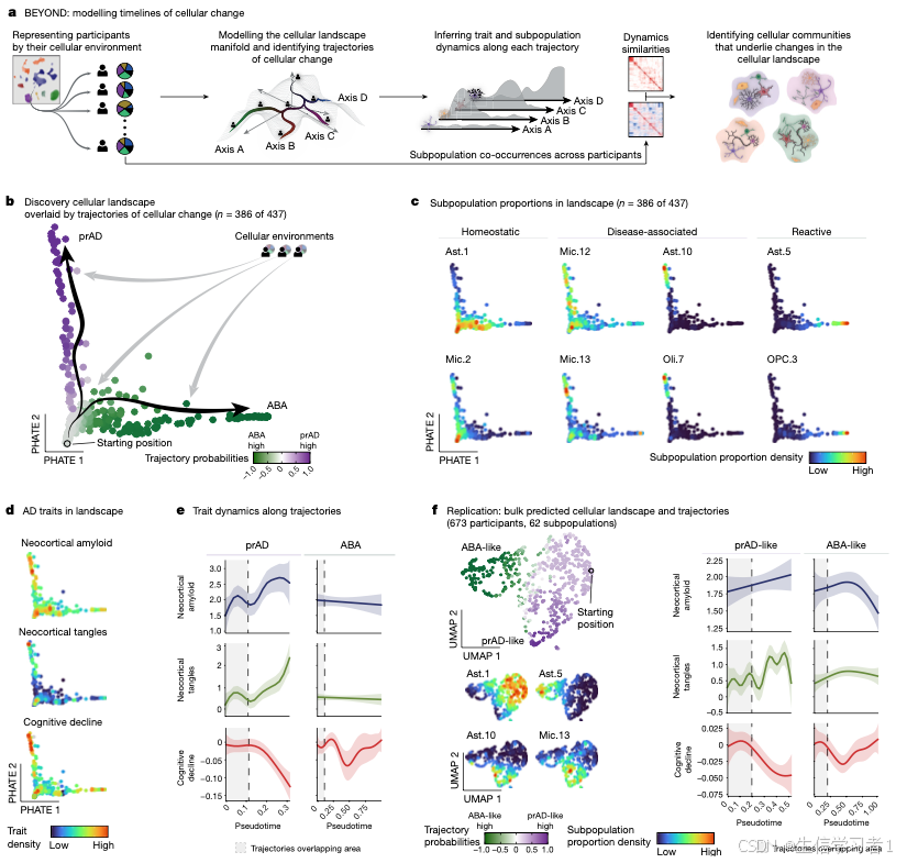
图6
source("5. Manuscript code/utils.R")


#####################################################################################################################
#                                           Figure 6 - Communities Structure                                        #
#####################################################################################################################

# ----------------------------------------------------------------------------------------------------------------- #
#                                       Panel A - Dynamics - states of interest                                     #
# ----------------------------------------------------------------------------------------------------------------- #
pdf(file.path(panel.path, "6A.pdf"), width=embed.width, height=embed.height.small)
for(states in state.dynamics.sets) {
  print(plot.dynamics(names(states), cols = states, overlap.pseudotime=.1, label=TRUE) +
    theme(strip.text = element_blank(),
          legend.position="none",
          axis.line = element_line(),
          axis.text.y = element_text()) +
    labs(x=NULL, y=NULL, title=NULL))
}
while (!is.null(dev.list()))  dev.off()
rm(states)


# ----------------------------------------------------------------------------------------------------------------- #
#                                      Panel B - Dynamics & adjacency matrices                                      #
# ----------------------------------------------------------------------------------------------------------------- #
library(dendextend)
communities   <- data$uns$communities
membership    <- split(data$var_names, data$var$community)
dynamics      <- communities$similarities$dynamics %>% `dimnames<-`(list(data$var_names, communities$dynamics.colnames))
corr          <- communities$similarities$correlation %>% `dimnames<-`(list(data$var_names, data$var_names))
dyn.adjacency <- communities$similarities$dynamics.adjacency %>% `dimnames<-`(list(data$var_names, data$var_names))


# States to annotate
mark.states <- c("Oli.2","Oli.3","Ast.1","Mic.2","OPC.1","Ast.3","Oli.6","Mic.12","Mic.13","Ast.10","Oli.7","Ast.5","OPC.3","Mic.6","Mic.7")

# Specify dynamics column-order: zero pseudotime in the middle
dynamics <- dynamics[,c(rev(colnames(dynamics)[grepl("ABA", colnames(dynamics))]),
                        colnames(dynamics)[grepl("prAD", colnames(dynamics))])]

# Hierarchically split community's membership, creating dynamics heatmap within each community/sub-community
hm.comms <- data$var %>% split(., as.character(.$community)) %>%
  lapply(., function(inner) {

    if(any(!is.na(inner$sub.community)))
      lst <- split(rownames(inner), as.character(inner$sub.community))
    else
      lst <- list(rownames(inner))

    lapply(lst, function(states) {
      mtx  <- dyn.adjacency[states,states] + corr[states,states]
      dend <- dendsort::dendsort(hclust(dist(mtx))) %>% as.dendrogram() %>% set("labels_to_character")

      prepare(Heatmap(dynamics[states,],
                      column_split =  factor(gsub("_.*", "", colnames(dynamics)), levels=c("ABA","prAD")),
                      cluster_rows = dend,
                      cluster_row_slices = F,
                      cluster_columns = F,
                      show_column_names = F,
                      show_row_names = T,
                      show_row_dend = T,
                      row_dend_width = unit(10,"pt"),
                      col = circlize::colorRamp2(seq(-4,4,length.out=21),
                                                 colorRampPalette(c("darkorchid4","white","#E65100"))(21)),
                      column_title = NULL,
                      row_names_side = "left",
                      column_gap = unit(1, "pt"),
                      right_annotation = rowAnnotation(states = anno_mark(which(rownames(mtx) %in% mark.states), intersect(rownames(mtx), mark.states)))))

    }) %>% unlist(., recursive=FALSE)
  })  %>% unlist(., recursive=FALSE)

hm.comms <- hm.comms %>% `[`(c("C3", "C1.C1.1", "C1.C1.2","C2.C2.2","C2.C2.3","C2.C2.1"))


# Create annotations of traits and pseudotime
df <- data$uns$trajectories$palantir$dynamics$pred.vals %>% py_to_r(.) %>%
  filter(feature %in% names(AD.traits)) %>%
  mutate(col=paste(trajectory, x, sep = "_"))

traits <- df %>% reshape2::dcast(col~feature, value.var="fit") %>% column_to_rownames("col")
hm.traits <- lapply(names(AD.traits), function(trait) {
  mtx <- t(traits[colnames(dynamics),trait])
  Heatmap(mtx,
          col = circlize::colorRamp2(seq(min(mtx), max(mtx), length.out=21),
                                     colorRampPalette(c("white", AD.traits.colors[[trait]]))(21)),
          name = AD.traits[[trait]],
          cluster_columns = F,
          height = unit(.25,"cm"),
          right_annotation = rowAnnotation(n=anno_mark(1, trait)))
}) %>% `names<-`(names(AD.traits))


pseudotime <- df %>% dplyr::select(col, x) %>% unique() %>% dcast(1~col, value.var = "x") %>% column_to_rownames("1") %>% `[`(,colnames(dynamics)) %>% as.matrix()
pseudotime <- Heatmap(pseudotime,
                      col = viridis::turbo(21),
                      name = "pseudotime",
                      show_row_names = F,
                      show_column_names = F,
                      cluster_columns = F,
                      height = unit(.25,"cm"),
                      right_annotation = rowAnnotation(n=anno_mark(1, "pseudotime")))

# Save figure of all heatmaps
pdf(file.path(panel.path, "6B.1.pdf"), width=embed.width*1.5, height=embed.height*2)
draw(modifyList(modifyList(hm.comms, hm.traits), list(ps=pseudotime))
     %>% base::Reduce("%v%", .), ht_gap = unit(1, "pt"))
while (!is.null(dev.list()))  dev.off()

# Retrieve state order to be used in composite adjacency matrix - Fig 5c
state.order <- do.call(rbind, lapply(hm.comms, function(hm) data.frame(comm = hm@name, state=rownames(hm@matrix)[row_order(hm)])))
rm(dynamics, hm.comms, df, traits, hm.traits, pseudotime)


# Plot dynamics adjacency and state-state correlations in lower/upper triangles
dyn.adjacency <- dyn.adjacency[state.order$state, state.order$state]
corr <- corr[state.order$state, state.order$state]

marks <- sapply(mark.states, function(s) which(rownames(dyn.adjacency) == s))
matrices <- list(dyn.adjacency, corr)
colors   <- list(circlize::colorRamp2(seq(0,1,length.out=21), colorRampPalette(c("white","salmon","red","firebrick4"))(21)),
                 circlize::colorRamp2(seq(-1,1,length.out=21), green2purple.less.white(21)))

pdf(file.path(path, "6B.2.pdf"), width=embed.width*2, height=embed.height*2)
for (i in 1:2) {
  Heatmap(
    matrices[[i]],
    row_split = state.order$comm,
    column_split = state.order$comm,
    cluster_rows = F,
    cluster_columns = F,
    col = colors[[i]],
    cell_fun = function(j, i, x, y, w, h, col) {
      if(i==j) grid.rect(x,y,w,h, gp = gpar(fill="black", col=NA))
    },
    column_title = NULL,
    row_title = NULL,
    show_heatmap_legend = F,
    show_row_names = F,
    show_column_names = F,
    row_gap = unit(2, "pt"),
    column_gap = unit(2, "pt"),
    right_annotation = rowAnnotation(states = anno_mark(marks, names(marks)))
  ) %>% draw()
}
while (!is.null(dev.list()))  dev.off()
rm(dyn.adjacency, corr, breaks, marks, mark.states, state.order, communities, membership, i, matrices, colors)


# ----------------------------------------------------------------------------------------------------------------- #
#                                           Panel C - Communities dynamics                                          #
# ----------------------------------------------------------------------------------------------------------------- #
pdf(file.path(panel.path, "6C.pdf"), width=embed.width, height=embed.height/2)
plot.dynamics(c("C1", "C2.2","C2.3","C3"), dynamics = data$uns$communities$dynamics, cols = comm.cols, legend.position = "none", overlap.pseudotime = .1) + labs(x=NULL, y=NULL)
while (!is.null(dev.list()))  dev.off()


# ----------------------------------------------------------------------------------------------------------------- #
#                                       Panel D - Communities trait associations                                    #
# ----------------------------------------------------------------------------------------------------------------- #
pdf(file.path(panel.path, "6D.pdf"), width=embed.width*.5, height=embed.height)
plot.trait.associations(py_to_r(data$uns$communities$trait.association) %>%
                          rename(state=covariate),
                        params = names(AD.traits),
                        show.only.significant = F,
                        column_labels = AD.traits,
                        column_names_rot = 45,
                        column_names_centered = T,
                        cluster_rows=F,
                        row_names_side = "left",
                        use_raster=F,
                        raster_quality = 10,
                        border=T)
while (!is.null(dev.list()))  dev.off()


# ----------------------------------------------------------------------------------------------------------------- #
#                                               Panel E - Community pathways                                        #
# ----------------------------------------------------------------------------------------------------------------- #

states <- data$var %>%
  mutate(grouping.by = recode(grouping.by, "Excitatory Neurons" = "excitatory","Inhibitory Neurons" = "inhibitory",
                              "Oligodendrocytes" = "oligodendrocytes", "Astrocyte" = "astrocytes","Microglia" = "microglia", "OPCs" = "opcs",
                              "Vascular Niche" = "endo") %>% as.character()) %>%
  rownames_to_column() %>%
  unstack(rowname~grouping.by)

pdf(file.path(panel.path, "6F.pdf"), width=embed.width, height=embed.height)
lapply(list(c("Mic.12","Mic.13"), c("OPC.1","Ast.3"), c("Ast.9","Ast.10","Oli.13")), function(vals)
  do.call(rbind, lapply(names(states), function(ct)
    h5read(data.extended, file.path(mapping[[ct]], "pa")) %>%
      filter(state %in% vals & direction == "upregulated") %>%
      dplyr::select(state, Description))) %>%
    split(., .$state) %>%
    lapply(., function(x) x$Description) %>%
    `[`(rev(vals)) %>%
    make_comb_mat %>%
    t %>%
    UpSet(set_order = vals,
          comb_order = order(comb_degree(.)),
          border=TRUE,
          width=unit(2,"cm"),
          top_annotation = NULL,
          right_annotation = upset_right_annotation(., gp = gpar(fill="grey80"))) %>%
    draw %>%
    grid.grabExpr) %>%
  plot_grid(plotlist = ., ncol = 1)
while (!is.null(dev.list()))  dev.off()


# ----------------------------------------------------------------------------------------------------------------- #
#                                               Panel E - Community pathways                                        #
# ----------------------------------------------------------------------------------------------------------------- #
clustered.pathways  <- openxlsx::read.xlsx("5. Manuscript code/data/community.pathways.xlsx", sheet = 1)
clustering.args     <- openxlsx::read.xlsx("5. Manuscript code/data/community.pathways.xlsx", sheet = 2, rowNames = T)
pathway.annotations <- openxlsx::read.xlsx("5. Manuscript code/data/figures.data.xlsx", sheet = "community.pathways")

settings <- expand.grid(rownames(clustering.args), c("upregulated")) %>%
  `colnames<-`(c("comm","dirc")) %>%
  filter(comm %in% c("C4.2","C4.3"))

pdf(file.path(path, "6F.pdf"), width=embed.width*2, height=embed.height*2)
for(i in 1:nrow(settings)) {
  message(i)
  comm = as.character(settings[i, "comm"])
  dirc = settings[i, "dirc"]

  # Load community clustered pathways as well as "raw" state-specific pathways
  states <- data$var %>%
    mutate(grouping.by = recode(grouping.by,
                                "Excitatory Neurons" = "excitatory","Inhibitory Neurons" = "inhibitory",
                                "Oligodendrocytes" = "oligodendrocytes", "Astrocyte" = "astrocytes",
                                "Microglia" = "microglia", "OPCs" = "opcs","Vascular Niche" = "endo") %>% as.character()) %>%
    filter(community == comm | sub.community == comm) %>%
    `[`(c("Mic.12","Mic.13","Ast.3","OPC.1","Ast.10","Oli.7","Ast.9","Mic.11"),) %>%
    rownames_to_column()
  states <- split(states, states$grouping.by) %>% lapply(., function(x) x$rowname)

  pathways <- do.call(rbind, lapply(names(states), function(ct)
    h5read(data.extended, file.path(mapping[[ct]], "pa")) %>% filter(state %in% states[[ct]])))

  pathways <- clustered.pathways %>%
    dplyr::select(-gene, -geneID) %>%
    tidyr::separate_rows(state, sep="/") %>%
    merge(., pathways,
          by.x = c("state","direction","ID", "Description"),
          by.y = c("state","direction","ID", "Description"),
          suffixes = c(".grouped",""))


  # Prepare state~pathways data for plotting
  df <- pathways %>% filter(direction == dirc) %>%
    dplyr::select("state","direction","Description","p.adjust","membership") %>%
    reshape2::dcast(membership+direction+Description~state, value.var = "p.adjust", fun.aggregate = mean)

  # Determine clustered pathways ordering in heatmap
  ord <- df[,-(1:3)] %>% mutate_all(~replace(., is.na(.), 2)) %>% as.matrix %>%
    Heatmap(show_row_dend = F, show_column_dend = F, row_split = df$membership) %>% prepare()
  row.ord <- row_order(ord)
  col.ord <- column_order(ord)

  # Plot clustered heatmap with pathway annotations
  row.splitting <- stack(row.ord) %>% arrange(values) %>% pull(ind)

  text <- pathway.annotations %>% filter(community == comm & direction == dirc) %>% tidyr::separate_rows(pathways, sep="/") %>% unstack(pathways~cluster)
  anno <- anno_textbox(align_to = row.splitting,
                       text = text,
                       gp = gpar(fontsize=12, col="black"),
                       background_gp = gpar(fill="grey95", col="grey80"),
                       max_width=unit(6, "cm"),
                       text_space = unit(8, "pt"))

  cols <- green2purple(3)
  if(dirc == "downregulated")
    cols <- cols[1:2]
  else
    cols <- rev(cols[2:3])
  draw(Heatmap(df[stack(row.ord)[[1]],-(1:3)][,col.ord] %>% as.matrix,
          col = cols,
          row_split = row.splitting,
          cluster_rows = F, cluster_columns = F, show_row_names = F,
          border=T, row_gap = unit(0,"pt"),
          na_col = "grey90",
          right_annotation = rowAnnotation(pathways=anno),
          height = unit(10,"cm"),
          width = unit(.4*length(col.ord), "cm")))

}
while (!is.null(dev.list()))  dev.off()


# ----------------------------------------------------------------------------------------------------------------- #
#                                               Panel G - Mic.13-Ast.10 colocalization                              #
# ----------------------------------------------------------------------------------------------------------------- #
cols <- list(`Early/ABA`=green2purple(5)[2], prAD=green2purple(5)[4])
df <- readRDS("3. Other analyses/data/ST.validation.rds")$mic13.ast10.colocalization %>%
  mutate(trajectory = case_when(trajectory %in% c("Early","ABA") ~ "Early/ABA", .default = trajectory))

pdf(file.path(panel.path, "6F.pdf"), width=embed.width.small*1.2, height=embed.height.small)
ggplot(df, aes(trajectory, cor, fill=trajectory)) +
  geom_boxplot(outlier.size = 0) +
  geom_point(aes(shape=is.sig)) +
  scale_fill_manual(values=cols) +
  scale_shape_manual(values = list("TRUE"=16, "FALSE"=1))+
  theme_classic()
while (!is.null(dev.list()))  dev.off()

# ----------------------------------------------------------------------------------------------------------------- #
#                                                 Panel H - Ast.10-Ast.5 exclusivity                                #
# ----------------------------------------------------------------------------------------------------------------- #
cols <- list(ABA=green2purple(5)[2], prAD=green2purple(5)[4], Early = "grey70")
df <- readRDS("3. Other analyses/data/ST.validation.rds")$ast10.ast5.colocalization


pdf(file.path(panel.path, "6H.1.pdf"), width=embed.width.small, height=embed.height)
df %>% pivot_longer(cols = c("Ast.10", "Ast.5"), names_to="state") %>%
  select(trajectory, state, value) %>%
  ggplot(aes(trajectory, value, fill=trajectory)) +
  geom_violin() +
  geom_point() +
  facet_wrap(~state, ncol=1, scales = "free") +
  theme_classic() +
  theme(strip.background = element_blank(),
        legend.position = "none") +
  scale_fill_manual(values = cols)
while (!is.null(dev.list()))  dev.off()


pdf(file.path(panel.path, "6H.2.pdf"), width=embed.width, height=embed.height)
ggplot(df %>% filter(trajectory != "Early"), aes(trajectory, `10.vs.5`, fill=trajectory)) +
  geom_boxplot(outlier.size = 0) +
  geom_point(aes(shape=is.sig)) +
  scale_fill_manual(values=cols) +
  scale_shape_manual(values = list("TRUE"=16, "FALSE"=1))+
  theme_classic()
while (!is.null(dev.list()))  dev.off()


#####################################################################################################################
#                                       Supp Figure 6 - Communities Structure                                       #
#####################################################################################################################

# ----------------------------------------------------------------------------------------------------------------- #
#                             Panel A - Dynamics - states of interest - including points                            #
# ----------------------------------------------------------------------------------------------------------------- #

pdf(file.path(panel.path, "s9A.pdf"), width=embed.width, height=embed.height.small)
for(states in state.dynamics.sets) {
  print(plot.dynamics(names(states), cols = states, overlap.pseudotime=.1, label=TRUE, include.points = TRUE) +
          theme(strip.text = element_blank(),
                legend.position="none",
                axis.line = element_line(),
                axis.text.y = element_text()) +
          labs(x=NULL, y=NULL, title=NULL))
}
while (!is.null(dev.list()))  dev.off()
rm(states)


# ----------------------------------------------------------------------------------------------------------------- #
#                                           Panel B -  Communities node graphs                                      #
# ----------------------------------------------------------------------------------------------------------------- #
library(ggraph)
library(tidygraph)

communities <- data$uns$communities
labelled <- c("Ast.1","Mic.2","Oli.3", "Mic.6","Mic.7","OPC.3","Ast.5","Mic.12","Mic.13","OPC.1","Oli.6","Ast.3","Oli.7","Ast.10")

graph <-
  # Convert similarity matrices to undirected flat edge dataframes
  lapply(c("correlation", "dynamics.adjacency"), function(n)
    communities$similarities[[n]] %>%
      `dimnames<-`(list(data$var_names, data$var_names)) %>%
      melt %>%
      filter(value != 0 & Var1 != Var2) %>%
      mutate(type=n)) %>%
  do.call(rbind, .) %>%

  # Convert to tidygraph - with workaround for duplicated edges
  as_tbl_graph(directed=FALSE) %>%
  activate(edges) %>%
  group_by(from, to, value, type) %>%
  filter(row_number() == 1) %>%
  ungroup() %>%

  # Append community information
  activate(nodes) %>%
  mutate(community = data$var[name, "community"],
         sub.community = data$var[name, "sub.community"],
         grouping.by = data$var[name,"grouping.by"],
         label = ifelse(name %in% labelled, name, NA_character_)) %>%
  activate(edges) %>%
  mutate(cross = .N()$community[from] != .N()$community[to]) %>%
  activate(nodes)


pos <- list(C1=c(0,0), C2 = c(-2, -.5), C3=c(2, -.5))
la <- lapply(names(pos), function(comm)
  graph %>% filter(community == comm) %>%
    activate(edges) %>%
    filter(abs(value) >= .1) %>%
    create_layout(layout = "graphopt") %>%
    mutate(across(c(x,y), ~scales::rescale(., c(-.5,.5))),
           x = x+pos[[comm]][1], y = y+pos[[comm]][2])
) %>% do.call(rbind, .) %>%
  column_to_rownames("name") %>%
  `[`(graph %>% pull(name),)


pdf(file.path(panel.path, "s9B.pdf"),width=3*1.5, height=3)
for(configuration in list(list("correlation", .2, TRUE),
                          list("correlation", .2, FALSE),
                          list("dynamics.adjacency", .2, TRUE),
                          list("dynamics.adjacency", .2, FALSE))) {

  # Subset edges based on configuration
  .sub <- graph %>% activate(edges) %>%
    filter(type == configuration[[1]] &
             abs(value) >= configuration[[2]] &
             cross == configuration[[3]]) %>%
    activate(nodes)

  p <- ggraph(.sub, layout = "manual", x=la$x, y=la$y)
  if (configuration[[3]]) # If plotting between community edges
    p <- p + geom_edge_fan(aes(colour = value, edge_width=abs(value)/50), n=10, alpha=.6)

  p <- p + ggforce::geom_mark_hull(
    aes(x, y, group = community),
    fill="grey90", concavity = 5, expand = unit(2, "mm"), alpha = .6)

  if(!configuration[[3]]) # If plotting within community edges
    p <- p + geom_edge_fan(aes(colour = value, edge_width=abs(value)/50), n=10, alpha=.6)

  if(configuration[[1]] == "correlation")
    p <- p + scale_edge_colour_gradient2(low=green2purple(2)[[1]], high = green2purple(2)[[2]], limit=c(-1,1))
  else
    p <- p + scale_edge_colour_gradient2(low="grey", high = "firebrick4", limit=c(0,1))

  p <- p +
    scale_edge_width_binned(range=c(.1, 1), breaks=c(.2,.4,.6,.8,1)) +
    geom_node_point(aes(fill=grouping.by), size=2, shape=21) +
    scale_fill_manual(values = cell.group.color) +
    geom_node_text(aes(filter = !is.na(label), label = label), colour = "black", repel = TRUE) +
    theme(panel.background = element_blank())

  print(p)
}
dev.off()
rm(p, configuration, la, pos, graph, labelled, communities)


# ----------------------------------------------------------------------------------------------------------------- #
#                                           Panel C - Communities dynamics                                          #
# ----------------------------------------------------------------------------------------------------------------- #
pdf(file.path(panel.path, "s9C.pdf"), width=embed.width, height=embed.height*1.5)
plot_grid(plot.dynamics(c("C1", "C2","C3"), dynamics = data$uns$communities$dynamics, cols = comm.cols, include.points = TRUE,  legend.position = c(3,3), overlap.pseudotime = .1) + labs(x=NULL, y=NULL),
          plot.dynamics(c("C1.1","C1.2"), dynamics = data$uns$communities$dynamics, cols = comm.cols, include.points = TRUE,legend.position = c(3,3), overlap.pseudotime = .1) + labs(x=NULL, y=NULL),
          plot.dynamics(c("C2.1","C2.2","C2.3"), dynamics = data$uns$communities$dynamics, cols = comm.cols, include.points = TRUE,legend.position = c(3,3), overlap.pseudotime = .1) + labs(x=NULL, y=NULL),
          ncol=1)
while (!is.null(dev.list()))  dev.off()


# ----------------------------------------------------------------------------------------------------------------- #
#                                       Panel D - Replication state dynamics                                        #
# ----------------------------------------------------------------------------------------------------------------- #
bulk <- anndata::read_h5ad("4. BEYOND/data/Celmod.subpopulation.proportion.h5ad")
pdf(file.path(panel.path, "s9D.pdf"), width=embed.width, height=embed.height.small)
for(states in state.dynamics.sets) {
  print(plot.dynamics(names(states), cols = states, data. = bulk, dynamics = bulk$uns$trajectories$dynamics, overlap.pseudotime=.2, label=TRUE, include.points = TRUE) +
          theme(strip.text = element_blank(),
                legend.position="none",
                axis.line = element_line(),
                axis.text.y = element_text()) +
          labs(x=NULL, y=NULL, title=NULL))}
while (!is.null(dev.list()))  dev.off()
rm(states, bulk)


# ----------------------------------------------------------------------------------------------------------------- #
#                                       Panel E - ST participants in landscape                                      #
# ----------------------------------------------------------------------------------------------------------------- #
cols <- list(ABA=green2purple(2)[1], prAD=green2purple(2)[2], Early = "grey30")

df <- data$obsm$X_core_phate %>% `colnames<-`(c("PHATE_1","PHATE_2")) %>% filter(!is.na(PHATE_1)) %>%
  merge(data$X[,c("Mic.13","Ast.10","Ast.5")], by.x="row.names", by.y="row.names") %>%
  merge(data.frame(data$uns$trajectories$palantir$branch.probs %>% py_to_r, pseudotime = data$uns$trajectories$palantir$pseudotime), by.x="Row.names", by.y="row.names") %>%
  merge(readRDS("3. Other analyses/data/ST.validation.state.signatures.rds") %>% select(trajectory, sample) %>% unique, by.x="Row.names", by.y="sample", all.x=TRUE) %>%
  arrange(!is.na(trajectory))

pdf(file.path(panel.path, "s9E.pdf"), width=embed.width, height=embed.height)
ggplot(df, aes(PHATE_1, PHATE_2, color=trajectory)) +
  geom_point() +
  ggrepel::geom_label_repel(aes(label=Row.names),data = df %>% filter(!is.na(trajectory))) +
  scale_color_manual(values = cols, na.value = "lightgrey") +
  theme_classic() +
  theme(axis.text = element_blank(),
        axis.ticks = element_blank(),
        legend.position = "none") +
  labs(x=NULL, y=NULL)
while (!is.null(dev.list()))  dev.off()


# ----------------------------------------------------------------------------------------------------------------- #
#                                       Panel F - Mic.13-Ast.10 spatial correlation                                 #
# ----------------------------------------------------------------------------------------------------------------- #
cols <- list(ABA=green2purple(5)[2], prAD=green2purple(5)[4], Early = "grey70")
df <- readRDS("3. Other analyses/data/ST.validation.state.signatures.rds") %>%
  arrange(trajectory, sample) %>% mutate(sample=paste(trajectory, sample))


pdf(file.path(panel.path, "s9F.pdf"), width=embed.height.small*length(unique(df$sample)), height=embed.height.small)
ggplot(df , aes(Mic.13, Ast.10, group="1")) +
  geom_point(size=.25, color="grey") +
  geom_smooth(method="lm", color="black") +
  facet_wrap(~sample, scales = "free", nrow=1) +
  theme_classic() +
  theme(strip.background = element_blank())
while (!is.null(dev.list()))  dev.off()


# ----------------------------------------------------------------------------------------------------------------- #
#                                       Panel G - Ast.10-Ast.5 spatial incompatibility                              #
# ----------------------------------------------------------------------------------------------------------------- #
cols <- list(Ast.5=green2purple(5)[2], Ast.10=green2purple(5)[4])
df <- readRDS("3. Other analyses/data/ST.validation.state.signatures.rds") %>%
  arrange(trajectory, sample) %>% mutate(sample=paste(trajectory, sample))

pdf(file.path(panel.path, "s9G.pdf"), width=embed.height.small*.8*length(unique(df$sample)), height=embed.height.small)
df %>% pivot_longer(cols = c("Ast.10","Ast.5"), names_to = "state") %>%
  arrange(trajectory) %>%
  ggplot(., aes(state, value, fill=state)) +
  geom_violin(draw_quantiles = c(0.25, 0.5, 0.75)) +
  facet_wrap(~sample, scales = "free", nrow=1) +
  theme_classic() +
  theme(strip.background = element_blank(),
        legend.position = "none") +
  scale_fill_manual(values = cols)
while (!is.null(dev.list()))  dev.off()
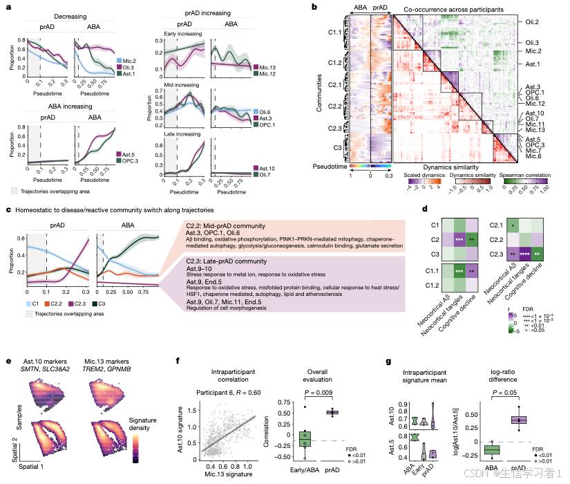


 被折叠的 条评论
为什么被折叠?
被折叠的 条评论
为什么被折叠?
 到【灌水乐园】发言


