吴恩达机器学习（六）—— ex2：Logistic Regression（MATLAB+Python）

最新推荐文章于 2021-08-29 18:47:42 发布

大彤小忆

最新推荐文章于 2021-08-29 18:47:42 发布

阅读量2k

点赞数 8

分类专栏：机器学习文章标签：机器学习

本文链接：https://blog.csdn.net/HUAI_BI_TONG/article/details/108423980

版权

机器学习专栏收录该内容

26 篇文章 98 订阅

订阅专栏

吴恩达机器学习系列内容的学习目录 $\rightarrow$ 吴恩达机器学习系列内容汇总。

本次练习对应的基础知识总结 $\rightarrow$ Logisitic回归和正则化。

本次练习对应的文档说明和提供的MATLAB代码 $\rightarrow$ 提取码：iuvr 。

本次练习对应的完整代码实现(MATLAB + Python版本) $\rightarrow$ Github链接。

一、Logistic回归

在本部分练习中，我们将建立一个Logistic回归模型，以预测学生是否被大学录取。
假设你是大学一个部门的管理人员，并且你想根据每位申请者的两次考试成绩来确定他们的录取机会。你拥有每位申请者的历史数据，可以用作Logistic回归的训练集。对于每个训练样本，你都有申请者的两次考试成绩以及录取决定。
我们的任务是建立一个分类模型，根据这两次考试成绩来估计申请者的录取概率。我们可以通过ex2.m中的代码框架完成本次练习。

1.1 可视化数据

在开始使用任何学习算法之前，最好尽可能可视化数据。在ex2.m的第一部分中，代码将加载数据并通过调用plotData函数将其显示在二维图上。
现在，我们将在plotData中完成代码，以使其显示如图1所示的图形，其中轴是两次考试成绩，并且正负两种样本用不同的标记表示。
完成plotData.m时需要填写以下代码：

% Find Indices of Positive and Negative Examples %找出正反例子的索引
pos = find(y==1); neg = find(y == 0);  %pos 和neg 分别是 y元素=1和0的所在的位置序号组成的向量
% Plot Examples
plot(X(pos, 1), X(pos, 2), 'k+','LineWidth', 2,'MarkerSize', 7); %x中对应y等于1的第一列和第二列
plot(X(neg, 1), X(neg, 2), 'ko', 'MarkerFaceColor', 'y','MarkerSize', 7);%将数据点以圆形、黄色实心填充

当运行ex2.m时，可以得到训练数据散点图如图1所示。在这里插入图片描述

图1 训练数据散点图

1.2 实现

1.2.1 热身练习：sigmoid函数

在开始实际的代价函数之前，请记住Logistic回归假设函数定义为： $h_{\theta }(x)=g(\theta ^{T}X)$

其中，函数 $g$ 是sigmoid函数，sigmoid函数公式为 $g(z)=\frac{1}{1+e^{-z}}$ 。
我们第一步是在sigmoid.m中实现此函数，以便程序的其余部分可以调用它，成后试着在MATLAB命令行中调用sigmoid（x）来测试一些值。对于x为较大的正值，S形应该接近1；对于x为较大的负值，S形应该接近0；计算sigmoid（0）应该恰好为0.5。
完成sigmoid.m时需要填写以下代码：

g = 1./(1+exp(-z));

1.2.2 代价函数和梯度

现在，我们将实现Logistic回归的代价函数和梯度。完成costFunction.m中的代码以返回代价和梯度。
Logistic回归中的代价函数为 $J(\theta )=-\frac{1}{m}\sum_{i=1}^{m}[y^{(i)}\times log(h_{\theta}(x^{(i)}))+(1-y^{(i)})\times log(1-h_{\theta}(x^{(i)}))]$

代价函数的梯度是一个与 $θ$ 长度相同的向量，其中第 $j$ 个元素（ $j = 0, 1 ， . . . ， n$ ）的定义如下： $\frac{\partial J(\theta )}{\partial \theta _{j}}=\frac{1}{m}\sum_{i=1}^{m}(h_{\theta }(x^{(i)})-y^{(i)} )x^{(i)}_{j}$

值得注意的是，虽然此梯度看上去与线性回归的梯度相同，但实际上公式不同，因为线性回归和Logistic回归对应的 $h_{\theta }(x)$ 不同。
完成costFunction.m时需要填写以下代码：

J=(1/m)*(-y'*log(sigmoid(X*theta))-(1-y')*log(1-sigmoid(X*theta)));
grad=(1/m)*X'*(sigmoid(X*theta)-y);

完成后，ex2.m将使用 $θ$ 的初始参数调用costFunction，我们应该看到代价约为0.693。

Cost at initial theta (zeros): 0.693147
Expected cost (approx): 0.693

1.2.3 利用fminunc学习参数

在ex1中，我们通过实现梯度下降找到了线性回归模型的最佳参数。当时我们编写了一个代价函数并计算了其梯度，然后相应地采取了梯度下降步骤。这次我们将使用名为fminunc的 MATLAB内置函数，而不是执行梯度下降步骤。
MATLAB的fminunc是一个寻找无约束函数最小值的优化求解器。对于Logistic回归，我们想使用参数 $θ$ 优化代价函数 $J (θ)$ 。
具体而言，在给定固定的数据集（X和y值）的情况下，将使用fminunc来找到Logistic回归代价函数的最佳参数 $θ$ 。我们将传递给fminunc以下输入：

我们正在尝试优化的参数的初始值；
一个函数，当给定训练集和特定的 $θ$ 时，该函数针对数据集（X，y）计算特定 $θ$ 时对应的Logistic回归代价和梯度。

在ex2.m中，已经编写了使用正确参数调用fminunc的代码。

% Set options for fminunc
options = optimset('GradObj', 'on', 'MaxIter', 400);
% Run fminunc to obtain the optimal theta
% This function will return theta and the cost
[theta, cost] = ...
fminunc(@(t)(costFunction(t, X, y)), initial theta, options);

在此代码段中，我们首先定义了与fminunc一起使用的选项。具体来说，我们将GradObj选项设置为on，这告诉fminunc，我们的函数同时返回代价和梯度，当最小化函数时允许fminunc使用梯度。此外，我们将MaxIter选项设置为400，使得fminunc在终止之前最多运行400步。
为了指定我们要最小化的实际函数，我们使用“short-hand”来指定 @(t)(costFunction(t,X,y)) 的函数。这将创建一个带有参数 $t$ 的函数，该函数将调用costFunction。这允许我们可以包装costFunction与fminunc一起使用。
如果正确完成了costFunction，fminunc将收敛于正确的优化参数并返回代价和 $θ$ 的最终值。注意，通过使用fminunc，我们不必自己编写任何循环，也不必像对梯度下降那样设置学习率，这一切都由fminunc完成，我们只需要提供一个计算代价和梯度的函数即可。
一旦fminunc完成，ex2.m将使用 $θ$ 的最佳参数调用costFunction函数，我们应该看到代价约为0.203。

Cost at theta found by fminunc: 0.203498
Expected cost (approx): 0.203
theta: 
 -25.161343 
 0.206232 
 0.201472 
Expected theta (approx):
 -25.161
 0.206
 0.201

然后，将使用最终的 $θ$ 值在训练数据上绘制决策边界，调用plotDecisionBoundary.m得到的结果如图2所示。
在这里插入图片描述

图2 带有决策边界的训练数据

1.2.4 评价Logistic回归

学习完参数后，我们可以使用模型预测一个特定的学生是否会被录取。对于考试1分数为45且考试2分数为85的学生，我们应该期望其录取概率为0.776。
评价我们找到的参数质量的另一种方法是看学习的模型在我们的训练集上预测的有多好。在这一部分，我们的任务是完成predict.m中的代码，通过给定的数据集和学习参数向量 $θ$ ，predict函数将产生“ 1”或“ 0”预测。
完成predict.m时需要填写以下代码：

p=round(sigmoid(X*theta)); %Round函数返回一个数值，该数值是按照指定的小数位数进行四舍五入运算的结果。
                           %如果round函数只有参数number,等同于digits 等于 0
                           %如果 digits 等于 0，则四舍五入到最接近的整数

完成predict.m中的代码后，ex2.m脚本将通过计算正确的样本百分比来报告分类器的训练精度，结果如下所示。

For a student with scores 45 and 85, we predict an admission probability of 0.776291
Expected value: 0.775 +/- 0.002

Train Accuracy: 89.000000
Expected accuracy (approx): 89.0

二、Logistic回归的正则化

在本部分练习中，我们将实现Logistic回归的正则化，以预测来自制造工厂的微芯片是否通过质量保证（QA）。在质量检查过程中，每个微芯片都要经过各种测试以确保其正常运行。
假设你是工厂的产品经理，并且在两次不同的测试中获得了某些微芯片的测试结果。从这两次测试中，你想确定应该接受还是拒绝微芯片。为了帮助你做出决定，你拥有过去微芯片测试结果的数据集，可以从中建立Logistic回归模型。
我们将使用另一个脚本ex2_reg.m来完成本部分练习。

2.1 可视化数据

与第一部分的练习类似，plotData用于生成如图3所示的图形，其中的轴是两次测试分数，正类（y = 1，接受）和负类（y = 0，拒绝）样本用不同的标记表示。在这里插入图片描述

图3 训练数据图

图3显示我们的数据集无法通过直线区分正、负样本。因此，Logistic回归的直接应用在此数据集上效果不佳，因为Logistic回归只能找到线性决策边界。

2.2 特征映射

更好地拟合数据的一种方法是从每个数据点创造更多的特征。在提供的函数mapFeature.m中，我们将把这些特征映射到所有 $x_{1}$ 和 $x_{2}$ 的多项式项，直到六次方。
$mapFeature(x)=\begin{bmatrix} 1\\ x_{1}\\ x_{2}\\ x_{1}^{2}\\ x_{1}x_{2}\\ x_{2}^{2}\\ x_{1}^{3}\\ \vdots \\ x_{1}x_{2^{5}}\\ x_{2}^{6} \end{bmatrix}$

由于此映射，我们的两个特征向量（两次QA测试的得分）已转换为28维向量。在此较高维特征向量上训练的Logistic回归分类器将具有更复杂的决策边界，并且在我们的二维图中绘制时将显示非线性。
尽管特征映射使我们能够构建更具表达力的分类器，但它也更容易过拟合。在下面的练习中，我们将实现正则化Logistic回归以拟合数据，并了解正则化如何帮助解决过度拟合问题。

2.3 代价函数和梯度

现在，我们将实现代码计算代价函数和梯度以进行Logistic回归的正则化。完成costFunctionReg.m中的代码以返回成本和梯度。
Logistic回归中的正则化成本函数为 $J(\theta)=\frac{1}{m}\sum_{i=1}^{m} [-y^{(i)}\times log(h_{\theta}(x^{(i)}))-(1-y^{(i)})\times log(1-h_{\theta}(x^{(i)}))]+\frac{\lambda }{2m} \sum_{j=1}^{n} \theta _{j}^{2}$

代价函数的梯度是一个向量，其中第 $j$ 个元素的定义如下：

$\begin{matrix} \frac{\partial J(\theta )}{\partial \theta _{0}}=\frac{1}{m}\sum_{i=1}^{m} (h _{\theta}(x^{(i)})-y^{(i)})x_{j}^{(i)}\ _{}\ _{}\ _{}\ _{}for\ _{}\ _{}j=0\ _{}\ _{}\ _{}\ _{}\ _{}\ _{}\ _{}\ _{}\ _{}\ _{}\ _{}\ _{}\ _{}\ _{}\\ \\ \frac{\partial J(\theta )}{\partial \theta _{j}}=\left (\frac{1}{m}\sum_{i=1}^{m} (h _{\theta}(x^{(i)})-y^{(i)})x_{j}^{(i)} \right )+\frac{\lambda }{m}\theta _{j}\ _{}\ _{}\ _{}\ _{}for\ _{}\ _{}j\geqslant 1 \end{matrix}$

完成costFunctionReg.m时需要填写以下代码：

theta_t=theta;
theta_t(1)=0; %不对theta0（theta1）进行惩罚
J=(1/m)*(-y'*log(sigmoid(X*theta))-(1-y')*log(1-sigmoid(X*theta)))+(lambda/(2*m))*sum(theta_t.^2);
grad=(1/m)*X'*(sigmoid(X*theta)-y)+(lambda/m)*theta_t;

完成后，ex2_reg.m将使用 $θ$ 的初始值（初始化为全零）调用costFunctionReg函数，我们可以看到代价约为0.693。

Cost at initial theta (zeros): 0.693147
Expected cost (approx): 0.693
Gradient at initial theta (zeros) - first five values only:
 0.008475 
 0.018788 
 0.000078 
 0.050345 
 0.011501 
Expected gradients (approx) - first five values only:
 0.0085
 0.0188
 0.0001
 0.0503
 0.0115

2.3.1 使用fminunc学习参数

与前面的部分相似，我们将使用fminunc来学习最佳参数 $θ$ 。如果我们正确完成了正则化Logistic回归的代价和梯度（costFunctionReg.m），则应该能够逐步遍历ex2_reg.m的下一部分，以使用fminunc学习参数 $θ$ 。

2.4 绘制决策边界

为了帮助我们可视化此分类器学习的模型，练习提供了函数plotDecisionBoundary.m，该函数绘制了将正负样本分开的（非线性）决策边界。在plotDecisionBoundary.m中，我们通过在均匀间隔的网格上计算分类器的预测值来绘制非线性决策边界，然后绘制预测从y = 0变为y =1的等高线图。
学习了参数 $θ$ 之后， ex2_reg.m中调用plotDecisionBoundary将绘制如图4的决策边界。
在这里插入图片描述

图4 具有决策边界的训练数据（λ= 1）

与ex2.m脚本类似，ex2_reg.m可以通过调用predict函数得到分类器的训练精度为83.1%。

Train Accuracy: 83.050847
Expected accuracy (with lambda = 1): 83.1 (approx)

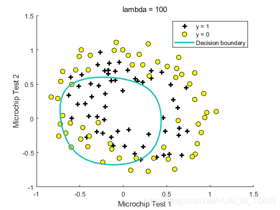
2.5 可选练习

在本部分练习中，我们将为数据集尝试不同的正则化参数，以了解正则化如何防止过度拟合。
随着 $λ$ 的变化，决策边界也在变化。 $λ$ 很小时，我们会发现分类器几乎可以正确地训练每个训练样本，但是会画出非常复杂的边界，从而使数据过度拟合（如图5）。使用较大的 $λ$ 时，我们会看到一个显示更简单的决策边界的图，该决策边界仍将正负样本之间很好地分开。但是，如果将 $λ$ 设置得太高，我们将无法很好地拟合，并且决策边界也无法很好地跟随数据，从而使数据拟合不足（如图6）。在这里插入图片描述

图5 未正则化（过度拟合）（λ= 0）
在这里插入图片描述

图6 正则化过多（欠拟合）（λ= 100）

三、MATLAB实现

3.1 ex2.m

%% Machine Learning Online Class - Exercise 2: Logistic Regression
%
%  Instructions
%  ------------
% 
%  This file contains code that helps you get started on the logistic
%  regression exercise. You will need to complete the following functions 
%  in this exericse:
%
%     sigmoid.m
%     costFunction.m
%     predict.m
%     costFunctionReg.m
%
%  For this exercise, you will not need to change any code in this file,
%  or any other files other than those mentioned above.
%

%% Initialization
clear ; close all; clc

%% Load Data
%  The first two columns contains the exam scores and the third column
%  contains the label.

data = load('ex2data1.txt');
X = data(:, [1, 2]); y = data(:, 3);

%% ==================== Part 1: Plotting ====================
%  We start the exercise by first plotting the data to understand the 
%  the problem we are working with.

fprintf(['Plotting data with + indicating (y = 1) examples and o ' ...
         'indicating (y = 0) examples.\n']);

plotData(X, y);

% Put some labels 
hold on;
% Labels and Legend
xlabel('Exam 1 score')
ylabel('Exam 2 score')

% Specified in plot order
legend('Admitted', 'Not admitted')  %对各种图标进行标注
hold off;

fprintf('\nProgram paused. Press enter to continue.\n');
pause;


%% ============ Part 2: Compute Cost and Gradient ============
%  In this part of the exercise, you will implement the cost and gradient
%  for logistic regression. You neeed to complete the code in 
%  costFunction.m

%  Setup the data matrix appropriately, and add ones for the intercept term
[m, n] = size(X);

% Add intercept term to x and X_test
X = [ones(m, 1) X];

% Initialize fitting parameters
initial_theta = zeros(n + 1, 1);

% Compute and display initial cost and gradient
[cost, grad] = costFunction(initial_theta, X, y);

fprintf('Cost at initial theta (zeros): %f\n', cost);
fprintf('Expected cost (approx): 0.693\n');
fprintf('Gradient at initial theta (zeros): \n');
fprintf(' %f \n', grad);
fprintf('Expected gradients (approx):\n -0.1000\n -12.0092\n -11.2628\n');

% Compute and display cost and gradient with non-zero theta
test_theta = [-24; 0.2; 0.2];
[cost, grad] = costFunction(test_theta, X, y);

fprintf('\nCost at test theta: %f\n', cost);
fprintf('Expected cost (approx): 0.218\n');
fprintf('Gradient at test theta: \n');
fprintf(' %f \n', grad);
fprintf('Expected gradients (approx):\n 0.043\n 2.566\n 2.647\n');

fprintf('\nProgram paused. Press enter to continue.\n');
pause;


%% ============= Part 3: Optimizing using fminunc  =============
%  In this exercise, you will use a built-in function (fminunc) to find the
%  optimal parameters theta.

%  Set options for fminunc
options = optimset('GradObj', 'on', 'MaxIter', 400); %设置所有参数及其值，未设置的为默认值 %GradObj:用户定义的目标函数的梯度 %MaxIter:最大迭代次数

%  Run fminunc to obtain the optimal theta
%  This function will return theta and the cost 
[theta, cost] = ...
	fminunc(@(t)(costFunction(t, X, y)), initial_theta, options);%输入参数为options,该参数的的作用包括是否使用用户自定义的梯度下降公式（GradObj）以及迭代次数（MaxIter）

% Print theta to screen
fprintf('Cost at theta found by fminunc: %f\n', cost);
fprintf('Expected cost (approx): 0.203\n');
fprintf('theta: \n');
fprintf(' %f \n', theta);
fprintf('Expected theta (approx):\n');
fprintf(' -25.161\n 0.206\n 0.201\n');

% Plot Boundary
plotDecisionBoundary(theta, X, y);

% Put some labels 
hold on;
% Labels and Legend
xlabel('Exam 1 score')
ylabel('Exam 2 score')

% Specified in plot order
legend('Admitted', 'Not admitted')
hold off;

fprintf('\nProgram paused. Press enter to continue.\n');
pause;

%% ============== Part 4: Predict and Accuracies ==============
%  After learning the parameters, you'll like to use it to predict the outcomes
%  on unseen data. In this part, you will use the logistic regression model
%  to predict the probability that a student with score 45 on exam 1 and 
%  score 85 on exam 2 will be admitted.
%
%  Furthermore, you will compute the training and test set accuracies of 
%  our model.
%
%  Your task is to complete the code in predict.m

%  Predict probability for a student with score 45 on exam 1 
%  and score 85 on exam 2 

prob = sigmoid([1 45 85] * theta);
fprintf(['For a student with scores 45 and 85, we predict an admission ' ...
         'probability of %f\n'], prob);
fprintf('Expected value: 0.775 +/- 0.002\n\n');

% Compute accuracy on our training set
p = predict(theta, X);

fprintf('Train Accuracy: %f\n', mean(double(p == y)) * 100);
fprintf('Expected accuracy (approx): 89.0\n');
fprintf('\n');

3.2 ex2_reg.m

%% Machine Learning Online Class - Exercise 2: Logistic Regression
%
%  Instructions
%  ------------
%
%  This file contains code that helps you get started on the second part
%  of the exercise which covers regularization with logistic regression.
%
%  You will need to complete the following functions in this exericse:
%
%     sigmoid.m
%     costFunction.m
%     predict.m
%     costFunctionReg.m
%
%  For this exercise, you will not need to change any code in this file,
%  or any other files other than those mentioned above.
%

%% Initialization
clear ; close all; clc

%% Load Data
%  The first two columns contains the X values and the third column
%  contains the label (y).

data = load('ex2data2.txt');
X = data(:, [1, 2]); y = data(:, 3);

plotData(X, y);

% Put some labels
hold on;

% Labels and Legend
xlabel('Microchip Test 1')
ylabel('Microchip Test 2')

% Specified in plot order
legend('y = 1', 'y = 0')
hold off;


%% =========== Part 1: Regularized Logistic Regression ============
%  In this part, you are given a dataset with data points that are not
%  linearly separable. However, you would still like to use logistic
%  regression to classify the data points.
%
%  To do so, you introduce more features to use -- in particular, you add
%  polynomial features to our data matrix (similar to polynomial
%  regression).
%

% Add Polynomial Features

% Note that mapFeature also adds a column of ones for us, so the intercept
% term is handled
X = mapFeature(X(:,1), X(:,2));

% Initialize fitting parameters
initial_theta = zeros(size(X, 2), 1);

% Set regularization parameter lambda to 1
lambda = 1;

% Compute and display initial cost and gradient for regularized logistic
% regression
[cost, grad] = costFunctionReg(initial_theta, X, y, lambda);

fprintf('Cost at initial theta (zeros): %f\n', cost);
fprintf('Expected cost (approx): 0.693\n');
fprintf('Gradient at initial theta (zeros) - first five values only:\n');
fprintf(' %f \n', grad(1:5));
fprintf('Expected gradients (approx) - first five values only:\n');
fprintf(' 0.0085\n 0.0188\n 0.0001\n 0.0503\n 0.0115\n');

fprintf('\nProgram paused. Press enter to continue.\n');
pause;

% Compute and display cost and gradient
% with all-ones theta and lambda = 10
test_theta = ones(size(X,2),1);
[cost, grad] = costFunctionReg(test_theta, X, y, 10);

fprintf('\nCost at test theta (with lambda = 10): %f\n', cost);
fprintf('Expected cost (approx): 3.16\n');
fprintf('Gradient at test theta - first five values only:\n');
fprintf(' %f \n', grad(1:5));
fprintf('Expected gradients (approx) - first five values only:\n');
fprintf(' 0.3460\n 0.1614\n 0.1948\n 0.2269\n 0.0922\n');

fprintf('\nProgram paused. Press enter to continue.\n');
pause;

%% ============= Part 2: Regularization and Accuracies =============
%  Optional Exercise:
%  In this part, you will get to try different values of lambda and
%  see how regularization affects the decision coundart
%
%  Try the following values of lambda (0, 1, 10, 100).
%
%  How does the decision boundary change when you vary lambda? How does
%  the training set accuracy vary?
%

% Initialize fitting parameters
initial_theta = zeros(size(X, 2), 1);

% Set regularization parameter lambda to 1 (you should vary this)
lambda = 1;

% Set Options
options = optimset('GradObj', 'on', 'MaxIter', 400);

% Optimize
[theta, J, exit_flag] = ...
	fminunc(@(t)(costFunctionReg(t, X, y, lambda)), initial_theta, options);

% Plot Boundary
plotDecisionBoundary(theta, X, y);
hold on;
title(sprintf('lambda = %g', lambda))

% Labels and Legend
xlabel('Microchip Test 1')
ylabel('Microchip Test 2')

legend('y = 1', 'y = 0', 'Decision boundary')
hold off;

% Compute accuracy on our training set
p = predict(theta, X);

fprintf('Train Accuracy: %f\n', mean(double(p == y)) * 100);
fprintf('Expected accuracy (with lambda = 1): 83.1 (approx)\n');

四、Python实现

4.1 ex2.py

import numpy as np
import matplotlib.pylab as plt
import scipy.optimize as op

# Load Data
data = np.loadtxt('ex2data1.txt', delimiter=',') #指定冒号作为分隔符(delimiter)
X = data[:, 0:2]
Y = data[:, 2]

# ==================== Part 1: Plotting ====================
print('Plotting data with + indicating (y = 1) examples and o indicating (y = 0) examples.')

# 绘制散点图像
def plotData(x, y):
    pos = np.where(y == 1)
    neg = np.where(y == 0)
    p1 = plt.scatter(x[pos, 0], x[pos, 1], marker='+', s=30, color='b')#scatter(x, y, 点的大小, 颜色，标记)绘制散点图
    p2 = plt.scatter(x[neg, 0], x[neg, 1], marker='o', s=30, color='y')
    plt.legend((p1, p2), ('Admitted', 'Not admitted'), loc='upper right', fontsize=8)
    plt.xlabel('Exam 1 score')
    plt.ylabel('Exam 2 score')
    plt.show()

plotData(X, Y)
_ = input('Press [Enter] to continue.')

# ============ Part 2: Compute Cost and Gradient ============
m, n = np.shape(X)
X = np.concatenate((np.ones((m, 1)), X), axis=1)  ## 这里的axis=1表示按照列进行合并(axis=0表示按照行进行合并)
init_theta = np.zeros((n+1,))

# sigmoid函数
def sigmoid(z):
    g = 1/(1+np.exp(-1*z))
    return g

# 计算损失函数和梯度函数
def costFunction(theta, x, y):
    m = np.size(y, 0)
    h = sigmoid(x.dot(theta))
    if np.sum(1-h < 1e-10) != 0:  #1-h < 1e-10相当于h > 0.99999999
        return np.inf  #np.inf 无穷大
    j = -1/m*(y.dot(np.log(h))+(1-y).dot(np.log(1-h)))
    return j

def gradFunction(theta, x, y):
    m = np.size(y, 0)
    grad = 1 / m * (x.T.dot(sigmoid(x.dot(theta)) - y))
    return grad

cost = costFunction(init_theta, X, Y)
grad = gradFunction(init_theta, X, Y)
print('Cost at initial theta (zeros): ', cost)
print('Gradient at initial theta (zeros): ', grad)
_ = input('Press [Enter] to continue.')

# ============= Part 3: Optimizing using fmin_bfgs  =============
result = op.minimize(costFunction, x0=init_theta, method='BFGS', jac=gradFunction, args=(X, Y)) #fun:求最小值的目标函数;x0:变量的初始猜测值;minimize是局部最优的解法;args:常数值（元组）;
                                                                                                #method:求极值的方法(BFGS逻辑回归法);jac:计算梯度向量的方法
theta = result.x
print('Cost at theta found by fmin_bfgs: ', result.fun) #result.fun为最小代价
print('theta: ', theta)

# 绘制图像
def plotDecisionBoundary(theta, x, y):
    pos = np.where(y == 1)
    neg = np.where(y == 0)
    p1 = plt.scatter(x[pos, 1], x[pos, 2], marker='+', s=60, color='r')
    p2 = plt.scatter(x[neg, 1], x[neg, 2], marker='o', s=60, color='y')
    plot_x = np.array([np.min(x[:, 1])-2, np.max(x[:, 1]+2)])
    plot_y = -1/theta[2]*(theta[1]*plot_x+theta[0])
    plt.plot(plot_x, plot_y)
    plt.legend((p1, p2), ('Admitted', 'Not admitted'), loc='upper right', fontsize=8)
    plt.xlabel('Exam 1 score')
    plt.ylabel('Exam 2 score')
    plt.show()

plotDecisionBoundary(theta, X, Y)
_ = input('Press [Enter] to continue.')

# ============== Part 4: Predict and Accuracies ==============
prob = sigmoid(np.array([1, 45, 85]).dot(theta))
print('For a student with scores 45 and 85, we predict an admission probability of: ', prob)

# 预测给定值
def predict(theta, x):
    m = np.size(X, 0)
    p = np.zeros((m,))
    pos = np.where(x.dot(theta) >= 0)
    neg = np.where(x.dot(theta) < 0)
    p[pos] = 1
    p[neg] = 0
    return p
p = predict(theta, X)
print('Train Accuracy: ', np.sum(p == Y)/np.size(Y, 0))

4.2 ex2_reg.py

import numpy as np
import matplotlib.pylab as plt
import scipy.optimize as op

# 加载数据
data = np.loadtxt('ex2data2.txt', delimiter=',')
X = data[:, 0:2]
Y = data[:, 2]

def plotData(x, y):
    pos = np.where(y == 1)
    neg = np.where(y == 0)
    p1 = plt.scatter(x[pos, 0], x[pos, 1], marker='+', s=50, color='b')
    p2 = plt.scatter(x[neg, 0], x[neg, 1], marker='o', s=50, color='y')
    plt.legend((p1, p2), ('Admitted', 'Not admitted'), loc='upper right', fontsize=8)
    plt.xlabel('Exam 1 score')
    plt.ylabel('Exam 2 score')
    plt.show()

plotData(X, Y)
_ = input('Press [Enter] to continue.')

# =========== Part 1: Regularized Logistic Regression ============
# 向高维扩展
def mapFeature(x1, x2):
    degree = 6
    col = int(degree*(degree+1)/2+degree+1) #28维
    out = np.ones((np.size(x1, 0), col))
    count = 1
    for i in range(1, degree+1):
        for j in range(i+1):
            out[:, count] = np.power(x1, i-j)*np.power(x2, j)
            count += 1
    return out

X = mapFeature(X[:, 0], X[:, 1])
init_theta = np.zeros((np.size(X, 1),))
lamd = 1

# sigmoid函数
def sigmoid(z):
    g = 1/(1+np.exp(-1*z))
    return g

# 损失函数
def costFuncReg(theta, x, y, lam):
    m = np.size(y, 0)
    h = sigmoid(x.dot(theta))
    j=-1/m*(y.dot(np.log(h))+(1-y).dot(np.log(1-h)))+lam/(2*m)*theta[1:].dot(theta[1:])
    return j

# 梯度函数
def gradFuncReg(theta, x, y, lam):
    m = np.size(y, 0)
    h = sigmoid(x.dot(theta))
    grad = np.zeros(np.size(theta, 0))
    grad[0] = 1/m*(x[:, 0].dot(h-y))
    grad[1:] = 1/m*(x[:, 1:].T.dot(h-y))+lam*theta[1:]/m
    return grad

cost = costFuncReg(init_theta, X, Y, lamd)
print('Cost at initial theta (zeros): ', cost)
_ = input('Press [Enter] to continue.')

# ============= Part 2: Regularization and Accuracies =============
init_theta = np.zeros((np.size(X, 1),))
lamd = 1
result = op.minimize(costFuncReg, x0=init_theta, method='BFGS', jac=gradFuncReg, args=(X, Y, lamd))
theta = result.x

def plotDecisionBoundary(theta, x, y):
    pos = np.where(y == 1)
    neg = np.where(y == 0)
    p1 = plt.scatter(x[pos, 1], x[pos, 2], marker='+', s=60, color='r')
    p2 = plt.scatter(x[neg, 1], x[neg, 2], marker='o', s=60, color='y')
    u = np.linspace(-1, 1.5, 50)
    v = np.linspace(-1, 1.5, 50)
    z = np.zeros((np.size(u, 0), np.size(v, 0)))
    for i in range(np.size(u, 0)):
        for j in range(np.size(v, 0)):
            z[i, j] = mapFeature(np.array([u[i]]), np.array([v[j]])).dot(theta)
    z = z.T
    [um, vm] = np.meshgrid(u, v)
    plt.contour(um, vm, z, levels=[0])
    plt.legend((p1, p2), ('Admitted', 'Not admitted'), loc='upper right', fontsize=8)
    plt.xlabel('Microchip Test 1')
    plt.ylabel('Microchip Test 2')
    plt.title('lambda = 1')
    plt.show()

plotDecisionBoundary(theta, X, Y)

# 预测给定值
def predict(theta, x):
    m = np.size(X, 0)
    p = np.zeros((m,))
    pos = np.where(x.dot(theta) >= 0)
    neg = np.where(x.dot(theta) < 0)
    p[pos] = 1
    p[neg] = 0
    return p

p = predict(theta, X)
print('Train Accuracy: ', np.sum(p == Y)/np.size(Y, 0))

大彤小忆

关注

8
点赞
踩
8

收藏

觉得还不错? 一键收藏
0
评论
吴恩达机器学习（六）—— ex2：Logistic Regression（MATLAB+Python）

一、Logistic回归       本次练习对应的文档说明和提供的MATLAB代码→\rightarrow→ 提取码：iuvr 。一、Logistic回归       在本部分练习中，我们将建立一个Logistic回归模型，以预测学生是否被大学录取。假设你是大学部门的管理员，并且您想根据每位申请人的两次考试成绩来确定他们的录取机会。您拥有以前申请人的历史数据.
复制链接

扫一扫