【论文学习3】LDAM：Learning Imbalanced Datasets with Label-Distribution-Aware Margin Loss

日期：2023/12/17
论文：Learning Imbalanced Datasets with Label-Distribution-Aware Margin Loss
链接：LDAM
会议：NeuraIPS 2019
参考：
[1] https://zhuanlan.zhihu.com/p/501900018

部分是参考内容中知乎里的部分

0 提前知识（自己不会的）

1. margin是数据点到决策边界的最小距离，每个类别的margin是该类别数据点到决策边界的最小margin。
2. SVM的目标就是找到一个决策边界，使得不同类别的数据点之间的margin最大，也就是最大化多个类别之间的margin。
3. Hinge loss是SVM使用来量化分类器性能的一个损失函数，定义为：$$L(y,f(x))=max(0,1-y\cdot f(x))$$其中$y\in [-1,1]$，$f(x)$是模型对样本x的预测。如果一个样本被正确分类并且足够远离决策边界，那么$y\cdot f(x)>1$，那么损失值为0； 如果被错误分类或者太接近决策边界，那么loss增加。
4. L2正则化是一种防止机器学习过拟合的技术，通常在损失函数加上一个正则化项来实现，该项与模型权重的平方成比例，目标就是惩罚大权重项，从而鼓励模型学习更平滑、泛化的特征表示，其定义如下$$L2=\lambda \sum _i{w}_i^2$$
5. Generalization error泛化误差是衡量一个模型在未见数据上的表现的重要指标，它常常与最小边际有关(minimum margin)，且与最小边际的倒数呈正相关关系。因为margin较小意味着决策边界与某些训练样本非常接近，导致模型对训练数据过敏，从而在新数据上表现不佳，换句话说，最小边际可能导致过拟合，自然就不能得到一个很好的泛化误差。

1 摘要

训练数据集出现严重的类不平衡问题会导致在实际应用中缺乏泛化性。该文设置了两种解决的算法：
1）基于标签分布的边界损失（Label-distribution-aware margin, LDAM);
2）延迟重新加权（Defers re-weighting, DRW)，既让模型学习初始特征表示，再进行re-weighting或re-sampling

2 Introduction

现在的2大common approaches就是re-weighting the losses或者 re-sampling the examples，但似乎两种方法都是在设计一种损失函数使得期望更接近测试集的分布，所以才能在头类和尾类之间的准确性上实现一个更好的平衡。但是我们对尾类信息知道的就很少，并且模型部署通常很大，所以就非常容易过拟合尾类数据，从而不能实现很好的泛化。（过拟合想到什么，正则化呀！！）

本文从正则化的角度入手，希望能狠狠正则化尾类数据，这样就能减少尾类数据的泛化误差，同时不牺牲模型对于头类数据的准确性。

Implementing this general idea requires a data-dependent or label-dependent regularizer — which in contrast to standard L2 regularization depends not only on the weight matrices but also on the labels — to differentiate frequent and minority classes

文中指出，L2正则化并不是一个很好的方法，因为它只取决于模型的权重，并没有取决于标签类型，所以并不能做到狠狠正则化尾类数据，它会将头类和尾类数据一起杀了。

Encouraging a large margin can be viewed as regularization, as standard generalization error bounds depend on the inverse of the minimum margin among all the examples.

本文的核心思想就是更大化尾类margin，从而起到一个正则化的效果

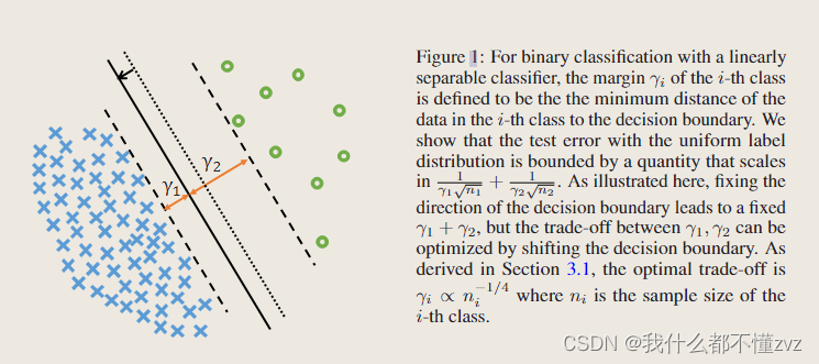
• 一个类的margin指的是该类所有样本到决策边界的最小距离，对于头类（蓝）和尾类（绿），如果我们有一个虚线的理想决策边界，那么${\gamma }_1={\gamma }_2$。但在class-imbalance任务中，模型对于尾类数据的特征表示往往是不够的，容易过拟合尾类，从而表现出很差的泛化能力。所以考虑降低对尾类的要求，从margin的角度来说，就是给予尾类更大的margin，所以实现的决策边界（实线）是更像头类靠近的。这就是本文的核心思想，至于偏移多少，后面会推导。
• 本文的modified loss function和re-sampling、re-weighting是相互独立的（orthogonal to…正交）

3 相关工作

3.1 Re-sampling

就是过采样和欠采样，暂时不学习采样方面。

3.2 Re-weighting

1） 基于各个类的频率的加权。但对于极端数据不平衡的情况可能导致深度学习难以优化。
2） 基于样本特性的加权。比如Focal loss基于样本预测难易程度，CBFocal loss基于梯度。

但是有研究也发现，如果没有正则项，逻辑回归会收敛到最大边距解决方案，既模型会过拟合尾类，从而忽略其他类的特征，此时weighting也没用。本文中，鼓励尾类有更大的边距，而不是收敛到最大边距。并且应用non-trivial L2正则化来实现最好的泛化性能。

3.3 Margin loss

Hinge loss通常提供最大边界，用于SVM。近期有large-margin softmax，angular softmax和additive margin softmax 被提出用于最小化类内变化，通过合并angular margin的思想来扩大类内边距。与这些论文中与类别无关的margin相反，此文的方法尽力为少数群体提供更大的margin。

3.4 Label shifting

Label shifting指训练数据集和测试数据集标签分布上的差异。举个医疗诊断的例子，夏天流感发病率低，而冬天流感发病率高，那么一个基于夏天数据训练的模型用于冬季，那么标签分布(流感or非流感）会发生显著变化，这就是label shift。
不平衡问题有时候也可以看作是迁移学习或domain adaption中的label shift问题，最大的困难就是评估标签的偏移，并且在这之后，运用re-sampling or re-weighting。在long-tail问题中，label shift是已知的，能否基于此做出更好的re-sampling or re-weighting？

3.5 Meta learning

.So far, we generally believe that our approaches that modify the losses are more computationally efficient than meta-learning based approaches.

4 主要方法（先忽略掉一些不懂的细节）

4.1 Loss的推导（不细节版）

1 定义误差
$$L_{bal}[f]=\underset{(x,y)\sim p_{bal}}{\mathrm{Pr}}[f(x{)}_y<\underset{l\ne y}{\max }f(x{)}_l]$$

• $f(x{)}_y$表示样本$x$预测为标签y的概率，其中y表示Ground Truth
• 括号内的含义是当预测为y类的概率是最大的，误差为0；当预测为其他类的概率大于预测为y类的概率，误差为1；
• 这是一个标准的0-1测试误差

2 定义margin
1）一个样本的margin
$$\gamma (x,y)=f(x{)}_y-\underset{j\ne y}{\max }f(x{)}_j$$

• 一个样本的margin定义为 它预测为GT的概率减去它预测为其他label的最大概率

2） 一个类的margin
$${\gamma }_j=\underset{i\in S_j}{\min }\gamma (x_i,y_i)$$

• 定义为该类样本点的最小margin就是该类margin

3）该数据集的margin
γ = m i n { γ 1 , γ 2 . . . γ k } \gamma = min\left\{\gamma_1,\gamma_2...\gamma_k\right\} γ=min{γ1​,γ2​...γk​}

• 定义为最小的类margin

3 测试集错误率上界
根据之前文献，当训练集和测试集有同样的数据分布时（既测试集也是不平衡的），测试集错误率上界与$C(F)、n和{\gamma }_{min}$有关，其中$C(F)$是分类器的评估方式。
$$imbalancedtesterror\le \frac{1}{{\gamma }_{min}}\sqrt{C(F)/n}$$
但是这样的上界就与标签分布无关，只与数据总数和最小边距有关。设计新的损失函数，针对不平衡数据集，如下
$$L_j[f]\le \frac{1}{{\gamma }_j}\sqrt{\frac{C(F)}{n_j}}+\frac{logn}{{\sqrt{n}}_j}$$
尾类数据量$n_j$很小，所以$\frac{1}{n_j}$很大，增大了损失值。但是$n_j$小的同时也增大了泛化误差。而类j的最小margin ${\gamma }_y$衡量的是分类器预测该类的预测准确率，增大margin，会增大准确率，既会降低泛化误差，也降低损失值，也就使得损失值保持在一定水平。这样就把标签分布也搬迁过来了，可以关注增大margin（n_j比较小）。总数据集上的loss就可以表示为
$$L_{bal}[f]\le \frac{1}{k}\sum _{j=1}^k\frac{1}{{\gamma }_j}\sqrt{\frac{C(F)}{n_j}}+\frac{logn}{{\sqrt{n}}_j}$$
那么margin该如何偏移呢？增大尾类margin的同时也会减小头类margin，这也是一个trade-off。当只有二类时，以下时factor的一个简化形式
$$\frac{1}{{\gamma }_1{\sqrt{n}}_1}+\frac{1}{{\gamma }_2{\sqrt{n}}_2}$$
当有一个偏移量$\delta$时，将问题转换为不等式
$$\frac{1}{{\gamma }_1{\sqrt{n}}_1}+\frac{1}{{\gamma }_2{\sqrt{n}}_2}\le \frac{1}{({\gamma }_1-\delta ){\sqrt{n}}_1}+\frac{1}{({\gamma }_2+\delta ){\sqrt{n}}_2}$$
将$\gamma$当作是n的参数，解的最优的margin为下式，其中C为常数
$${\gamma }_1=\frac{C}{n_1^{1/4}},and{\gamma }_2=\frac{C}{n_2^{1/4}}$$

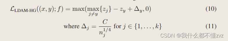
4 Loss形式
hinge loss 形式

CE loss 形式

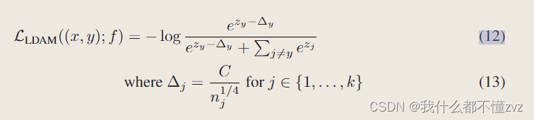
• 注意其中只有$z_y$减去了margin

4.2 Deferred Re-balancing Optimization Schedule

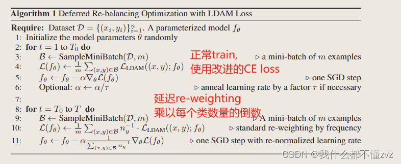
好处：

1. 训练初期不进行re-weighting，可以让模型更好学习到每个类别的特征，而不是过早聚焦与尾类，从而影响其泛化能力。
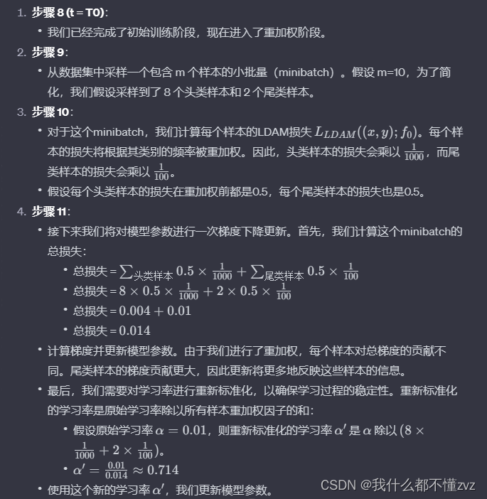
2. 后期引入re-weighting，让模型关注尾类，使得尾类数据有更大的权重。第11步缩放更新学习率来保持训练过程的稳定性。（以下是一个example）
   

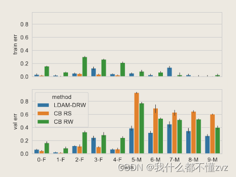
5 看看怎么做消融的

1. 实验方法

2. 两个数据集、不同imbalance ratio(难度)、不同steps、主要和class balanced比较

3. 不同loss和schedule组合

4. 展示在头类、尾类的错误率

6 代码

https://github.com/kaidic/LDAM-DRW/tree/master

class LDAMLoss(nn.Module):  
    def __init__(self, cls_num_list, max_m=0.5, weight=None, s=30):
        '''
        :param cls_num_list : 每个类别样本个数
        :param max_m : LDAM中最大margin参数,default =0.5
        :param weight : 
        :param s : 缩放因子,控制logits的范围
        '''
        super(LDAMLoss, self).__init__()
        m_list = 1.0 / np.sqrt(np.sqrt(cls_num_list)) # n_j 四次方根的倒数
        m_list = m_list * (max_m / np.max(m_list)) # 归一化，C相当于 max_m/ np.max(m_list)，确保没有大于max_m的

        m_list = torch.FloatTensor(m_list).cuda()
        self.m_list = m_list
        assert s > 0
        self.s = s
        self.weight = weight

    def forward(self, x, target):
        x = x.cuda()
        target = target.cuda()
        index = torch.zeros_like(x, dtype=torch.uint8).cuda() # 创建一个跟X一样的tensor
        index.scatter_(1, target.data.view(-1, 1), 1)   # 将每一行对应的target的序号设为1，其余保持为0
        index_float = index.type(torch.FloatTensor).cuda()

        batch_m = torch.matmul(self.m_list[None, :], index_float.transpose(0,1)) # 矩阵乘法，不同类别有不同的margin
        batch_m = batch_m.view((-1, 1)) # 变形之后，每一行与一个margin相减
        x_m = x - batch_m   
    
        output = torch.where(index, x_m, x) # 只有GT类会与margin相减
        return F.cross_entropy(self.s*output, target, weight=self.weight) # 通过一个缩放因子来放大logits，从而在使用softmax函数时增加计算结果的稳定性
    

# Demo to create LDAMLoss and validate with x and target
cls_num_list = [100, 10]  # Number of samples per class
ldam_loss = LDAMLoss(cls_num_list)
# logits output by the model for a batch of 2 samples
x = torch.tensor([[-1.5, 0.5], 
                  [0.2, -0.8]])

# true class labels for the batch
target = torch.tensor([0, 1])
# Calculate loss
loss = ldam_loss(x, target)
print(loss.item())