【人工智能学习之手写数字识别K-means聚类算法的Python实现示例及损失设计】

爱睡懒觉的焦糖玛奇朵

于 2024-06-25 09:45:55 发布

阅读量875

点赞数 24

分类专栏：人工智能学习笔记文章标签：人工智能算法学习

本文链接：https://blog.csdn.net/Jiagym/article/details/139647585

版权

人工智能学习笔记专栏收录该内容

17 篇文章 0 订阅

订阅专栏

【人工智能学习之手写数字识别K-means聚类算法的Python 实现示例】

1 前期准备
2 多分类交叉熵损失函数
3 CenterLoss中心点损失
4 ArcSoftmax损失

1 前期准备

1.1 所需模块

from torch import nn
import torch
from torchvision import datasets,transforms
from torch.utils.data import DataLoader
import matplotlib.pyplot as plt
# matplotlib版本不同需要调整
import matplotlib
matplotlib.use('TkAgg')

DEVICE = torch.device("cuda" if torch.cuda.is_available() else "cpu")

报错的话可以参考：TypeError: int() argument must be a string, a bytes-like object or a number, not ‘KeyboardModifier‘

1.2 下载数据集

直接下载手写数字的训练集

# 下载训练集
train_data = datasets.MNIST("data/",train=True,transform=transforms.ToTensor(),download=True)
train_loader = DataLoader(train_data,batch_size=600,shuffle=True)

1.3 全连接网络

因为手写数字识别很简单，直接使用全连接网络即可。
不过我们可以使用一些比较新的技术比如Mish()。
感兴趣的朋友也可以使用Relu()或者其它激活函数尝试，效果不是特别好，聚类比较随意。
在这里插入图片描述

class Net(nn.Module):
    def __init__(self):
        super().__init__()
        self.fc1 = nn.Sequential(
            nn.Linear(28*28*1,512,bias=False),
            nn.BatchNorm1d(512),
            nn.Mish(),
            nn.Linear(512,256,bias=False),
            nn.BatchNorm1d(256),
            nn.Mish(),
            nn.Linear(256,128,bias=False),
            nn.BatchNorm1d(128),
            nn.Mish(),
            nn.Linear(128,2),
        )
        self.fc2 = nn.Sequential(
            nn.Linear(2,10),
        )
    def forward(self,x):
        feature = self.fc1(x)
        cls_out = self.fc2(feature)
        return feature,cls_out

1.4 可视化2维特征

将特征分类可视化

# 可视化2维特征
def visualize(feature,labels,epoch):
    plt.ion()
    c = ["#ff0000","#ffff00","#00ff00","#00ffff","#0000ff",
         "#ff00ff","#990000","#999900","#009900","#009999"]
    plt.clf()
    for i in range(10):
        plt.plot(feature[labels==i,0],feature[labels==i,1],".",c=c[i])
    plt.legend(["0","1","2","3","4","5","6","7","8","9"],loc="upper right")
    plt.title("epoch=%d" % epoch)
    plt.savefig("images02/epoch=%d.jpg"%epoch)
    plt.draw()
    plt.pause(0.001)

2 多分类交叉熵损失函数

我们先使用多分类交叉熵损失函数，它可以衡量两个概率分布之间的距离
在深度学习中：概率分布=特征分布

if __name__ == '__main__':
    net = Net().to(DEVICE)
    loss_func = nn.CrossEntropyLoss()
    opt = torch.optim.Adam(net.parameters())
    EPOCH = 10000
    for epoch in range(EPOCH):
        feature_loader = []
        labels_loader = []
        for i,(img,label) in enumerate(train_loader):
            img = img.reshape(-1,28*28).to(DEVICE)
            label_ = label.to(DEVICE)

            feature,cls_out = net(img)

            loss = loss_func(cls_out,label_)

            opt.zero_grad()
            loss.backward()
            opt.step()

            feature_loader.append(feature)
            labels_loader.append(label)

            if i%10==0:
                print(f"epoch:{epoch},batch:{i},loss:{loss.item()}")
        features = torch.cat(feature_loader,0)
        labels = torch.cat(labels_loader)
        visualize(features.data.cpu().numpy(),labels.data.cpu().numpy(),epoch=epoch)

可以发现刚开始分布还比较混乱：
在这里插入图片描述
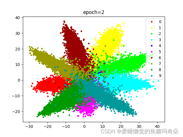
随着损失下降逐渐开始聚合。

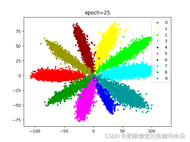
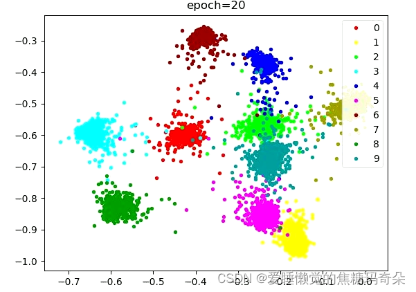
可以看到训练到八十次过后效果已经非常明显了。

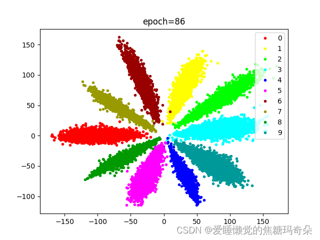
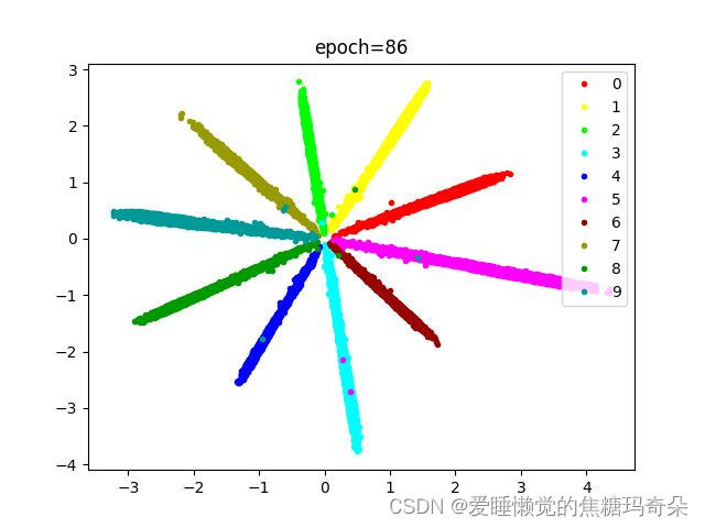
那么可不可以更优化一些呢，比如下图这样？

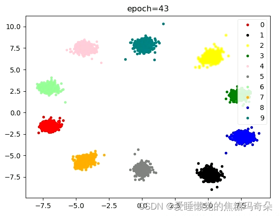
这就需要确定一个中心点让网络向那个方向收敛。

3 CenterLoss中心点损失

在这里插入图片描述
理解案例：

import torch
# 拟定一些参数
data = torch.Tensor([[3,4],[5,6],[7,8],[9,8],[6,5]])
label = torch.Tensor([0,0,1,0,1])
center = torch.Tensor([[1,1],[2,2]])
# 用label索引center进行扩充[[1,1],[1,1],[2,2],[1,1],[2,2]]
center_exp = center.index_select(dim=0,index=label.long())
print(center_exp)
# 统计label的类别
count = torch.histc(label,bins=2,min=0,max=1)
print(count)
# 用label索引count获取每部分的权重
count_exp = count.index_select(dim=0,index=label.long())
print(count_exp)
# 中心点公式
center_loss = torch.sum(torch.div(torch.sqrt(torch.sum(torch.pow(data-center_exp,2),dim=1)),count_exp))
print(center_loss)

中心点损失代码：

class CenterLoss(nn.Module):
    def __init__(self,cls_num,feature_num):
        super().__init__()
        self.cls_num = cls_num
        self.center = nn.Parameter(torch.randn(cls_num,feature_num))
    def forward(self,xs,ys):
        center_exp = self.center.index_select(dim=0, index=ys.long())
        count = torch.histc(ys, bins=self.cls_num, min=0, max=self.cls_num-1)
        count_exp = count.index_select(dim=0, index=ys.long())
        center_loss = torch.sum(torch.div(torch.sqrt(torch.sum(torch.pow(xs - center_exp, 2), dim=1)), count_exp))
        return center_loss

神经网络伪代码：

class MainNet(nn.Module):
    def __init__(self):
        super().__init__()
        self.hidden_layer = nn.Sequential(
            nn.Linear(784,120),
            nn.Mish(),
            nn.Linear(120,2)
        )
        self.output_layer = nn.Sequential(
            nn.Linear(2,10)
        )
        self.center_loss_layer = CenterLoss(10,2)
        self.crossEntropyLoss = nn.CrossEntropyLoss()
    def forward(self,xs):
        features = self.hidden_layer(xs)
        outputs = self.output_layer(features)
        return features,outputs

    def getLoss(self,outputs,features,labels):
        loss_cls = self.crossEntropyLoss(outputs,labels)
        loss_center = self.center_loss_layer(features,labels)
        loss = loss_cls + loss_center
        return loss

当然，网络也可以换成卷积，效果会更好一些。
卷积网络代码：

class VGGnet_pro(nn.Module):
    def __init__(self):
        super().__init__()
        self.center_loss_layer = CenterLoss(10, 2)
        self.crossEntropyLoss = nn.CrossEntropyLoss()

        self.conv_res = nn.Sequential(
            nn.Conv2d(64, 64, 1, 2, 0, bias=False),
            nn.BatchNorm2d(64),
        )
        self.conv_layer1 = nn.Sequential(
            nn.Conv2d(1, 64, 7, 2, 3, bias=False),
            nn.BatchNorm2d(64),
            nn.Mish(),
            nn.MaxPool2d(3, 2, 1)
        )

        self.conv_layer2 = nn.Sequential(
            nn.Conv2d(64, 128, 1, 1, 0, bias=False),
            nn.BatchNorm2d(128),
            nn.Mish(),
            nn.Conv2d(128, 128, 3, 1, 1, groups=128, bias=False),
            nn.BatchNorm2d(128),
            nn.Mish(),
            nn.Conv2d(128, 64, 1, 1, 0, bias=False),
            nn.BatchNorm2d(64),
            nn.Mish(),
        )
        self.conv_layer3 = nn.Sequential(
            nn.Conv2d(64, 64, 3, 2, 1, bias=False),
            nn.BatchNorm2d(64),
            nn.Mish(),
            nn.Conv2d(64, 64, 3, 1, 1, bias=False),
            nn.BatchNorm2d(64),
        )
        self.conv_layer4 = nn.Sequential(
            nn.Conv2d(64, 64, 3, 1, 1, bias=False),
            nn.BatchNorm2d(64),
            nn.Mish(),
            nn.Conv2d(64, 64, 3, 1, 1, bias=False),
            nn.BatchNorm2d(64),
            nn.Mish(),
            nn.Conv2d(64, 64, 3, 1, 1, bias=False),
            nn.BatchNorm2d(64),
            nn.Mish(),
            nn.AvgPool2d(4, 1)
        )
        self.classifier_xy = nn.Sequential(
            nn.Linear(64, 2)
        )
        self.classifier = nn.Sequential(
            nn.Linear(2, 10)
        )

    def forward(self, x):
        x = self.conv_layer1(x)

        res = self.conv_res(x)
        x = self.conv_layer2(x)
        x = self.conv_layer3(x)
        x = F.mish(x + res)

        x = self.conv_layer4(x)

        x = x.reshape(x.shape[0], -1)
        feature = self.classifier_xy(x)
        cls_out = self.classifier(feature)

        return feature, cls_out

    def getLoss(self, outputs, features, labels):
        loss_cls = self.crossEntropyLoss(outputs, labels)
        loss_center = self.center_loss_layer(features, labels)
        loss = loss_cls * 0.999 + loss_center * 0.001
        return loss

训练代码中只需要修改损失函数即可：

loss = net.getLoss(cls_out, feature, label_)

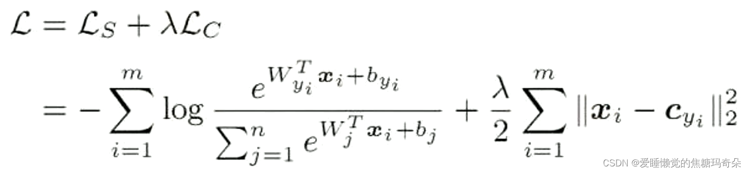
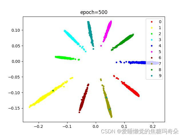
4 ArcSoftmax损失

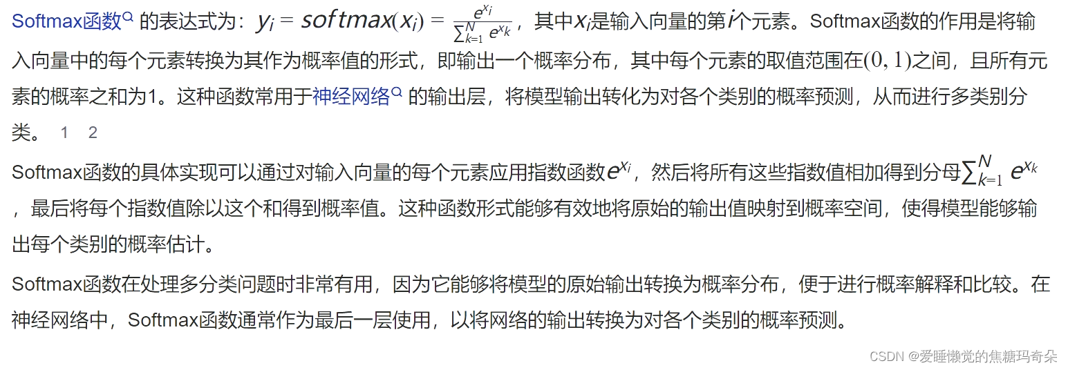
softmax函数大家都很熟悉，在此就不赘述了，不清楚的可以简单看一下下图。
在这里插入图片描述
Arc-SoftmaxLoss = Arc-Softmax + NLLLoss。
softmax 是通过角度分类的，Arc-Softmax 加宽了角度间的分界线，从而达到加大类间距的目的。

Arc-Softmax（加大 θ 角度）公式：
在这里插入图片描述
Arc-Softmax代码：

class ArcSoftmax(nn.Module):
    def __init__(self, feature_dim, cls_dim=10):
        super().__init__()
        self.w = nn.Parameter(torch.randn(feature_dim, cls_dim))

    def forward(self, feature, m=0.5, s=10):
        x = F.normalize(feature, dim=1)
        w = F.normalize(self.w, dim=0)
        cos = torch.matmul(x, w) / 10  #防止梯度爆炸 /10 
        a = torch.acos(cos)
        top = torch.exp(s * torch.cos(a + m))
        down = torch.sum(torch.exp(s * torch.cos(a)), dim=1, keepdim=True) - torch.exp(s * torch.cos(a)) + top
        out = torch.log(top/down)
        return out

网络代码：
Arc-Softmax可以直接替换分类的全连接层。

class VGGnet_pro(nn.Module):
    def __init__(self):
        super().__init__()
        self.center_loss_layer = CenterLoss(10, 2)
        self.crossEntropyLoss = nn.CrossEntropyLoss()
        self.arc_softmax = ArcSoftmax(2,10)
        self.nll_loss = nn.NLLLoss()

        self.conv_res = nn.Sequential(
            nn.Conv2d(64, 64, 1, 2, 0, bias=False),
            nn.BatchNorm2d(64),
        )
        self.conv_layer1 = nn.Sequential(
            nn.Conv2d(1, 64, 7, 2, 3, bias=False),
            nn.BatchNorm2d(64),
            nn.Mish(),
            nn.MaxPool2d(3, 2, 1)
        )

        self.conv_layer2 = nn.Sequential(
            nn.Conv2d(64, 128, 1, 1, 0, bias=False),
            nn.BatchNorm2d(128),
            nn.Mish(),
            nn.Conv2d(128, 128, 3, 1, 1, groups=128, bias=False),
            nn.BatchNorm2d(128),
            nn.Mish(),
            nn.Conv2d(128, 64, 1, 1, 0, bias=False),
            nn.BatchNorm2d(64),
            nn.Mish(),
        )
        self.conv_layer3 = nn.Sequential(
            nn.Conv2d(64, 64, 3, 2, 1, bias=False),
            nn.BatchNorm2d(64),
            nn.Mish(),
            nn.Conv2d(64, 64, 3, 1, 1, bias=False),
            nn.BatchNorm2d(64),
        )
        self.conv_layer4 = nn.Sequential(
            nn.Conv2d(64, 64, 3, 1, 1, bias=False),
            nn.BatchNorm2d(64),
            nn.Mish(),
            nn.Conv2d(64, 64, 3, 1, 1, bias=False),
            nn.BatchNorm2d(64),
            nn.Mish(),
            nn.Conv2d(64, 64, 3, 1, 1, bias=False),
            nn.BatchNorm2d(64),
            nn.Mish(),
            nn.AvgPool2d(4, 1)
        )
        self.classifier_xy = nn.Sequential(
            nn.Linear(64, 2)
        )
        self.classifier = nn.Sequential(
            nn.Linear(2, 10)
        )

    def forward(self, x):
        x = self.conv_layer1(x)

        res = self.conv_res(x)
        x = self.conv_layer2(x)
        x = self.conv_layer3(x)
        x = F.mish(x + res)

        x = self.conv_layer4(x)

        x = x.reshape(x.shape[0], -1)
        feature = self.classifier_xy(x)
        # cls_out = self.classifier(feature)
        out = self.arc_softmax(feature)

        # return feature, cls_out
        return feature, out

    def getLoss(self, outputs, features, labels):
        loss_cls = self.crossEntropyLoss(outputs, labels)
        loss_center = self.center_loss_layer(features, labels)
        loss = loss_cls * 0.999 + loss_center * 0.001
        return loss

    def getSoftmaxLoss(self, outputs, labels):
        return self.nll_loss(outputs,labels)

    def getTwoLoss(self, outputs, features, labels):
        loss_cls = self.getSoftmaxLoss(outputs, labels)
        loss_center = self.center_loss_layer(features, labels)
        loss = loss_cls * 0.999 + loss_center * 0.001
        return loss

同样，训练代码也只需要更改损失：

loss = net.getSoftmaxLoss(cls_out,label_)
loss = net.getTwoLoss(cls_out, feature, label_)

SoftmaxLoss的效果：
在这里插入图片描述
SoftmaxLoss+CenterLoss的效果：

爱睡懒觉的焦糖玛奇朵

关注

24
点赞
踩
12

收藏

觉得还不错? 一键收藏
0
评论
【人工智能学习之手写数字识别K-means聚类算法的Python实现示例及损失设计】

softmax 是通过角度分类的，Arc-Softmax 加宽了角度间的分界线，从而达到加大类间距的目的。感兴趣的朋友也可以使用Relu()或者其它激活函数尝试，效果不是特别好，聚类比较随意。softmax函数大家都很熟悉，在此就不赘述了，不清楚的可以简单看一下下图。我们先使用多分类交叉熵损失函数，它可以衡量两个概率分布之间的距离。不过我们可以使用一些比较新的技术比如Mish()。Arc-Softmax可以直接替换分类的全连接层。当然，网络也可以换成卷积，效果会更好一些。在深度学习中：概率分布=特征分布。
复制链接

扫一扫

专栏目录