Classify grayscale images by using common Machine Learning techniques

Classify grayscale images by using common Machine Learning techniques

Pengwei Yang
krysertim@gmail.com
SCSLab The University of Sydney J12/1 Cleveland St Sydney, NSW 2006 Australia

Introduction:

Machine learning consists of a set of algorithms that allow computers to perform automatical
learn like humans. Reliable and repeatable experimental results could be obtained due to data
analysis, and predictions will be accordingly made. There are many algorithms that can be
seen in machine learning, such as classification, regression, decision trees, clustering etc. In
terms of different learning methods, it can be mainly divided into supervised learning,
unsupervised learning, semi-supervised learning and reinforcement learning. The key idea is
to generalise training samples to get more accurate results. As for machine learning, the most
important factor is to describe the characteristics of the data and have enough data to train the
model. However, when processing data, there are bound to be some problems, it might due to
data deficiencies (insufficient data flow, large data noise, incomplete data functions, etc.) or
inappropriately selected algorithms. Therefore, it is necessary to use data preprocessing
technology or superimpose multiple data classifiers to continuously optimise and find the
most suitable training method.
In the era of data explosion, large amount of data needs to be processed every day. Artificial
intelligence is aimed to facilitate the completion of simple, boring and repetitive tasks, as a
result of that, saving energies could be used to improve other parts of information technology.
The main function of machine learning is to use some algorithms that allow computers to
learn automatically, summarise data and build data models, so as to obtain reliable and
repeatable results, and make predictions. In the decision-making area, we might better seek
potential opportunities and avoid risks. Machine learning is now widely used in government,
new energy, transportation, financial services, healthcare and other fields. After all, artificial
intelligence will shape our future more powerfully than any other innovation in this century.
Machine learning will change each industry and change our daily life as well.

Methods:

Pre-processing techniques:

Principal component analysis, also known as PCA, is the most popular dimensionality reduction method. The key idea of this method is considered to project the data into a new set of dimensions that is smaller than the original space, which means that PCA captures the critical part of data variance and ignores less important data variance(Abdi & Williams, 2010).
Normalisation, also called min-max scaling, is usually used to avoid the influences taken by the dominance of attributes over attributes with small values. The main idea of this method is to transform the original values of attributes into a new range(e.g. [0,1]). It has a significant effect, especially on distance-based Machine Learning algorithms.
Classifier methods:

1. Nearest Neighbour

The KNN algorithm needs to remember all the training examples and use a distance metric to find the training example that is closest to it. Then, the class labels of the nearest neighbours will serve as the predicted labels for new examples. The value of k is a key factor in prediction accuracy. It is effective to measure the weight of neighbours whether in classification or regression. The key idea is that closer neighbours have more weight than distant neighbours(H. et al., 2016).

Features:

1. Often very accurate
2. Slow for big datasets(examples)
3. Not effective for high-dimensional data(dimensionality reduction might solve this problem, but is not used in this report)
4. Sensitive to the number of neighbours, result from that, we choose n(i.e. neighbour number) as one of the hyperparameters

2. Decision Tree

A decision tree is a special tree structure that consists of a decision graph and possible outcomes to aid in decision making. Decision tree is one of the predictive models in machine learning. The key idea of this top-down learning model is a recursive divide-and-conquer approach(H. et al., 2016). Each node in the tree represents an object, each branch path represents a possible attribute value, and each leaf node corresponds to a root node to a leaf node. Traverse the value of the object represented by the path. A decision tree has only one output, and the algorithm is usually used to solve classification problems.
The measure of evaluating purity is called information gain, and it is based on another measure called entropy. The smaller the entropy, the higher the purity of the dataset and the higher the information gain.
If we grow a decision tree to perfectly classify the training set, the decision tree may become too specific and overfit the data, tree pruning could be used to avoid overfitting. There are two main strategies of tree pruning:
Pre-pruning - stop growing until the tree reaches the point where it perfectly classifies the training data.
Post-pruning - fully grow the tree so that it covers the training data perfectly, then prune it.
In general, post-pruning is preferred in practice.
Different post-pruning methods such as
• Subtree replacement
• Subtree feeding
• Convert trees to rules, then pruning them(H. et al., 2016)

Features:

1. Wellknown Machine Learning method and easy to implement
2. The key idea of DT is recursive divide-and-conquer process
3. Easy to understand due to visualisation
4. The implementation process is to select the best attribute according to the information gain
5. Use pruning to prevent overfitting

3. SVM

A support vector machine is a linear classifier with the largest margin in the feature space, which distinguishes it from a perceptron. SVMs include kernel tricks, which make them essentially non-linear classifiers(H. et al., 2016). The learning strategy of SVM is to maximise the interval, which can be formalised as an optimization algorithm for solving convex quadratic programming.

Features:

1. Very popular classification method
2. Introduce parameter C for trading off the relative importance of maximizing the margin and fitting the training data
3. Transform data into a higher dimensional space that is more likely to be linearly separable.
4. Introduce kernel function to do the calculations in the original rather than new higher-dimensional space.

4. Random forest (Ensemble)
   Random Forest combines Bagging and the single Decision Tree classifier. On the basis of building numerous Decision Tree models using Bagging ensemble method, the selection of random attributes is further added to the training process of the decision tree classifier. The traditional decision tree selects an optimal attribute among all the candidate attributes of the current node when selecting the attributes to be divided; while in RF, each node of the base decision tree is randomly selected from the set of candidate attributes of the node(H. et al., 2016). Choose a subset of k attributes, and then select an optimal attribute from this subset for partitioning. The selection of the number of attributes k is quite important.

Features:

1. Use Bagging (Key Idea: Guided Aggregation) method.
2. Use a decision tree as its base classifier
3. As the number of its base classifiers increases, the correlation increases
4. Its performance depends on the correlation between each base classifier and its base classifiers
5. Can run efficiently on large datasets and process input samples with high-dimensional features without dimensionality reduction.

Experiments and Results: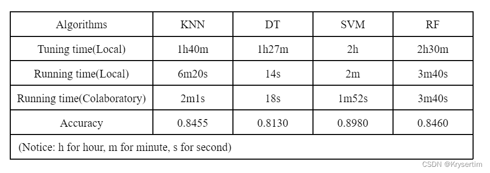

In light of above table, compared with other models, it is apparent that Support Vector Machine has the best accuracy(0.8980) and less running time(2min). On the contrary, K-Nearest Neighbour, which has the longest running time among the classifiers, needs 6 minutes and 20 seconds for building a model and predicting labels. And the accuracy of K-Nearest Neighbour is 0.8455, which is similar to the accuracy of Random Forest(0.8460). Additionally, Decision Tree has the shortest running time(14s) and the worst accuracy(0.8130).

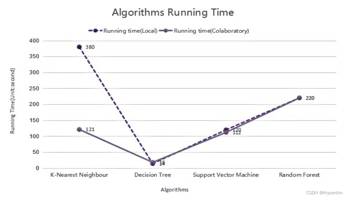
In terms of in-depth analysis, firstly, with regard to Decision Tree and Random Forest, the single Decision Tree model has the shortest running time among all classifiers, which is shown in the above line chart. And it is understandable that Random Forest has more running time. One possible reason is that a Random Forest classifier contains numerous base classifiers(i.e. Fully growth Decision Tree). And it is reasonable that the Random Forest classifier has a higher accuracy because the accuracy of its base classifier is higher than 50%. Apart from that, we use an additional preprocessing method, PCA(i.e. Principal Component Analysis), to reduce the dimensionality in order to have a shorter hyperparameter tuning time. Result from that, the accuracy of Random Forest might be influenced. In regard to the lowest accuracy of the single Decision Tree classifier, although we try to tune the depth of the tree(i.e. Pre-pruning) to avoid overfitting problems, it still has worse performance compared with other classifiers.
Secondly, with respect to the result(i.e. Running time based on local computation) of the K-Nearest Neighbour classifier, it can be seen as a time-consuming method, which can be clearly identified in the above line chart. When we input thirty thousand training data, the computer separately calculates the distance between the new example and each of the training data. As a result of that, it might cost lots of time. In addition to that, according to its accuracy, it has good accuracy which is similar to Random Forest.

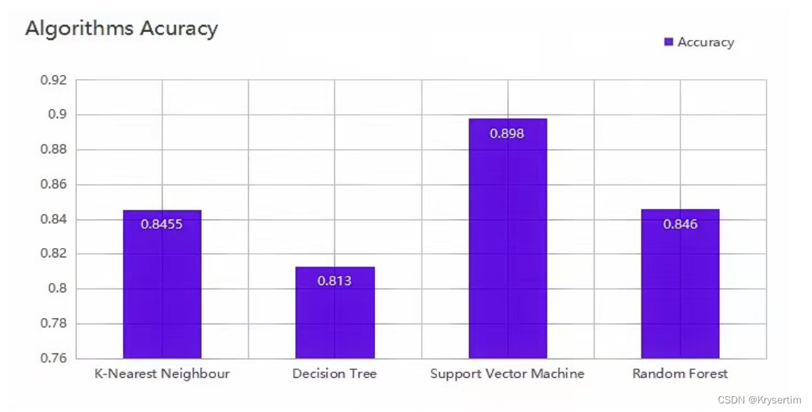
Thirdly, according to the results of the Support Vector Machine classifier, it is easily discovered that the SVM method has significantly better accuracy among all classifiers, which is clearly shown in the above bar chart. This case might due to the introduction of parameter C, which could be used to trade off the relative importance of maximizing the margin and fitting the training data, and the introduction of the kernel function, which could be used to effectively compute in high dimensional space. As for time consumption, SVM has a moderate running time compared with other classifiers.
Additionally, for the step of tuning hyperparameters, we use grid search which is based on eight-fold cross-validation to find the best combination of hyperparameters. And we tune the parameters(e.g. Set a sensible interval of numerical hyperparameters) to make sure the step of hyperparameter tunning is not very time-consuming. As for the hyperparameter selection, we choose several key parameters which could highly influence the model accuracy.
To sum up, after finely tuning hyperparameters, the Support Vector Machine classifier has the best performance while the single Decision Tree has the worst performance. Besides, K-Nearest Neighbour and the Random Forest classifiers have moderate performance but a longer running time compared with the single Decision Tree model.

Conclusion

After analysing the results of all classifiers, we find that SVM(i.e. Support Vector Machine) has the best performance. It might due to the introduction of parameter C and kernel function, which let SVM become an effective method when dealing with high dimensional data. Besides, the K-Nearest Neighbour model has a moderate performance with a long-running time because this method is ineffective for high-dimensional data and slow for big datasets. Apart from that, the single Decision Tree has the shortest running time but the worst performance, using an ensemble method like the Random Forest model might have the better performance.
There still exist several parts that need us to improve. For instance, we only use the grid-search method once for each kind of classifier in this assignment. In the future, we could narrow the range of hyperparameters to find better combinations of hyperparameters, which could be used to build a model with higher accuracy. Besides, we select several main hyperparameters to tune, namely the number of K and two kinds of distance calculational methods in the K-Nearest Neighbour classifier, depth of the tree and different criteria(i.e. Entropy, Gini) in the single Decision Tree model, three types of kernel functions and C parameter in the Support Vector Machine, the amount of base classifier and the quantity of subset of features in the Random Forest model. Apart from these parameters, there have more parameters that deserve us to do further study.

References

Abdi, & Williams, L. J. (2010). Principal component analysis. Wiley Interdisciplinary Reviews. Computational Statistics, 2(4), 433–459. doi: 10.1002/wics.101
Witten, I. H. (Ian H. ., Frank, E., Hall, M. A., & Pal, C. J. (2016). Data mining practical machine learning tools and techniques (4th ed.). Amsterdam: Elsevier.

Appendix

Code Instruction

We divide our code into several cells, and each kind of our classifier model includes several cells. Codes of each classifier could be run separately, and each classifier could upload its own test output file with the same name(i.e. test_output) after running its own part of codes. An important thing is that before running the whole code, the notebook file should be set in the root folder, and the root folder must contain two folders(i.e. Input folder and Output folder). By the way, the running time of grid-search of each classifier might be quite long, so the relevant codes could be jumped over and it will not influence the running of the later codes.

Hardware Environment

Local Environment:

CPU: Intel Core i7-6700

Software Environment：

Version of Python: Python 3
Used Packages: Pandas, Sklearn

#Four kinds of classifiers are separately shown below, SVM classifier is our best model.
#1.K-Nearest Neighbour##########################################################################################################
import pandas as pd

#Reading training data:
data_td = pd.read_csv('./Input/train/train.csv') #Reading the file of training data
d_ta_feature = data_td.loc[:, "v1":"v784"].to_numpy() #Take features of traning data
d_ta_label = data_td.loc[:, 'label'].to_numpy() #Take labels of training data

X_ta = d_ta_feature
y_ta = d_ta_label

#Normilisation for training data
from sklearn.preprocessing import MinMaxScaler #Use min-max scaling method
tool = MinMaxScaler() 
tool.fit(X_ta) #Calculate the min and the max value of the training data
X_ta_n = tool.transform(X_ta) 

#Grid search based on KNN
'''
Hyperparameters:
n for the number of neighbour, p for different kinds of distance calculational methods
In order to reduce the computational complexity, 
we choose n<=10, and we set interval 3(i.e. n=1,4,7,10)
As for hyperparameter p: p=1 -> Manhattan distance, p=2 -> Euclidean distance
'''
param_grid = {'n_neighbors': list(range(1,11,3)), 'p': [1, 2]} 
#Call the function of gridsearch based on cross-validation
from sklearn.model_selection import GridSearchCV 
#Call the function of KNN
from sklearn.neighbors import KNeighborsClassifier 
#8-fold cross-validation
gd_knn = GridSearchCV(KNeighborsClassifier(), param_grid, cv=8, return_train_score=False)
gd_knn.fit(X_ta_n, y_ta)
print("best hyperparameter: {}".format(gd_knn.best_params_))
#Best hyperparameter:{'n_neighbors': 4, 'p': 1}

#Reading test dataset
data_td = pd.read_csv('./Input/test/test_input.csv') #Reading the file of test data
d_te_feature = data_td.loc[:, "v1":"v784"].to_numpy() #Take features of test data
X_te = d_te_feature

#Normalisation for test data
from sklearn.preprocessing import MinMaxScaler
tool = MinMaxScaler() 
tool.fit(X_te)
X_te_n = tool.transform(X_te) 

#Build KNN model based on best hyperparameters('n_neighbors': 4, 'p': 1)
from sklearn.neighbors import KNeighborsClassifier
model_knn = KNeighborsClassifier(n_neighbors=4, p=1)
model_knn.fit(X_ta_n, y_ta) #Build KNN model using training data
y_pd = model_knn.predict(X_te_n) #Use the best model predict labels of test data
op = pd.DataFrame(y_pd, columns = ['label']) #Input values to a column which named label
#Upload the file
op.to_csv('./Output/test_output.csv', sep=",", float_format='%d', index_label="id") 
'''
RESULTS:
Running time-> 6m20s(Local) 2m1s(Colaboratory)
Accuracy    -> 0.84550
'''```

```python
#2.Decision Tree###############################################################################################################
import pandas as pd

#Reading training data:
data_td = pd.read_csv('./Input/train/train.csv') #Reading the file of training data
d_ta_feature = data_td.loc[:, "v1":"v784"].to_numpy() #Take features of traning data
d_ta_label = data_td.loc[:, 'label'].to_numpy() #Take labels of training data

X_ta = d_ta_feature
y_ta = d_ta_label

#Normalisation for training data 
from sklearn.preprocessing import MinMaxScaler #Use min-max scaling method
tool = MinMaxScaler()
tool.fit(X_ta) #Calculate the min and the max value of the training data
X_ta_n = tool.transform(X_ta) 

#Find the depth of the tree which is fully growth
#In order to set the number in the step of grid search
from sklearn.tree import DecisionTreeClassifier #Call the function of decision tree
t = DecisionTreeClassifier(random_state=42)
t.fit(X_ta_n, y_ta) #Build a fully growth decision tree model using training data
print(t.get_depth()) 
#Get the max_depth of tree-->37
```python
#Grid search based on DecisionTree
'''
Hyperparameters:
1.criterion(i.e.calculation based on Gini impurity or information gain)
2.max_depth->We already know the depth of fully growth tree is 37, 
consider of the computational complexity, we set interval as 5
'''
p_g = {'criterion': ['gini', 'entropy'], 'max_depth': range(2,38,5)}
#Call the function of gridsearch based on cross-validation
from sklearn.model_selection import GridSearchCV 
#8-fold cross-validation
gd_dt = GridSearchCV(DecisionTreeClassifier(), p_g, cv=8, return_train_score=False) 
gd_dt.fit(X_ta_n, y_ta)
print("best hyperparameter: {}".format(gd_dt.best_params_))
#Best hyperparameter:{'criterion': 'entropy', 'max_depth': 12}

import pandas as pd
#Reading test dataset
data_td = pd.read_csv('./Input/test/test_input.csv') #Reading the file of test data
d_te_feature = data_td.loc[:, "v1":"v784"].to_numpy() #Take features of test data
X_te = d_te_feature

#Normalisation for test data
from sklearn.preprocessing import MinMaxScaler
tool = MinMaxScaler() 
tool.fit(X_te)
X_te_n = tool.transform(X_te) 

#Build DecisionTree model based on best hyperparameters{'criterion': 'entropy', 'max_depth': 12}
from sklearn.tree import DecisionTreeClassifier 
model_DT = DecisionTreeClassifier(criterion='entropy', max_depth=12, random_state=42)
model_DT.fit(X_ta_n, y_ta) #Build DecisionTree model using training data
y_pd = model_DT.predict(X_te_n) #Use the best model predict labels of test data
op = pd.DataFrame(y_pd, columns = ['label']) #Input values to a column which named label
#Upload the file
op.to_csv('./Output/test_output.csv', sep=",", float_format='%d', index_label="id") 
'''
RESULTS:
Running time-> 14s(Local) 18s(Colaboratory)
Accuracy    -> 0.81300
'''

#3.Support Vector Machine【Our best model】##############################################################################################
import pandas as pd

#Reading training data:
data_td = pd.read_csv('./Input/train/train.csv') #Reading the file of training data
d_ta_feature = data_td.loc[:, "v1":"v784"].to_numpy() #Take features of traning data
d_ta_label = data_td.loc[:, 'label'].to_numpy() #Take labels of training data

X_ta = d_ta_feature
y_ta = d_ta_label

#Normalisation for training data 
from sklearn.preprocessing import MinMaxScaler #Use min-max scaling method
tool = MinMaxScaler() 
tool.fit(X_ta) #Calculate the min and the max value of the training data
X_ta_n = tool.transform(X_ta) 

#Grid search based on SVM
'''
Hyperparameters:
1.kernel->different kernel functions
2.C for trading off the relative importance of maximizing the margin and fitting the training data.
Large C: more emphasis on minimizing the training error than maximizing the margin.
Consider of the computational complexity, we only choose three values of C :0.1,1,10.
(The Latter one is ten times than the former one, which could allow a significant difference 
between these models)
'''
p_g = {'kernel': ['linear', 'poly', 'rbf'], 'C':[0.1, 1, 10]}
#Call the function of gridsearch based on cross-validation
from sklearn.model_selection import GridSearchCV 
from sklearn.svm import SVC #Call the function of SVM
grid_search = GridSearchCV(SVC(), p_g, cv=8, return_train_score=False) #8-fold cross-validation
grid_search.fit(X_ta_n, y_ta)
print("best hyperparameter: {}".format(grid_search.best_params_))
#Best hyperparameter: {'C': 10, 'kernel': 'rbf'}

#Reading test dataset
data_td = pd.read_csv('./Input/test/test_input.csv')
d_te_feature = data_td.loc[:, "v1":"v784"].to_numpy()
X_te = d_te_feature

#Normalisation for test data
from sklearn.preprocessing import MinMaxScaler
tool = MinMaxScaler() 
tool.fit(X_te)
X_te_n = tool.transform(X_te) 

#Build SVM model based on best hyperparameters{'C': 10, 'kernel': 'rbf'}
from sklearn.svm import SVC
model_svm = SVC(C=10, kernel="rbf")
model_svm.fit(X_ta_n, y_ta) #Build SVM model using training data
y_pd = model_svm.predict(X_te_n) #Use the best model predict labels of test data
op = pd.DataFrame(y_pd, columns = ['label']) #Input values to a column which named label
#Upload the file
op.to_csv('./Output/test_output.csv', sep=",", float_format='%d', index_label="id") 
'''
RESULTS:
Running time-> 2min(Local) 1m52s(Colaboratory)
Accuracy    -> 0.89800
'''

#4.Random Forest(Based on PCA)########################################################################################################
import pandas as pd

#reading training and test data
data_ta = pd.read_csv('./Input/train/train.csv') #Reading the file of training data
y_ta = data_ta.loc[:, 'label'].to_numpy() 
data_te = pd.read_csv('./Input/test/test_input.csv') #Reading the file of test data

#PCA for training and test data
from sklearn.decomposition import PCA #Call the function of PCA
pca=PCA(n_components=0.95) #Choose 95% variance
#Concatenate traning and test data
all_da = pd.concat((data_ta.loc[:,'v1':'v784'],data_te.loc[:,'v1':'v784'])) 
all_da_P = pca.fit_transform(all_da) #Using PCA to all data

X_ta_P = all_da_P[:data_ta.shape[0]] #Extract training data
X_te_P = all_da_P[data_ta.shape[0]:] #Extract test data
print("Reduced shape of training data: {}".format(str(X_ta_P.shape)))
print("Reduced shape of test data: {}".format(str(X_te_P.shape)))
'''
Print content:
Reduced shape of training data: (30000, 187)
Reduced shape of test data: (5000, 187)
'''

#Normalisation for training and test data
from sklearn.preprocessing import MinMaxScaler #Use min-max scaling method
tool = MinMaxScaler() 
tool.fit(X_ta_P) #Calculate the min and the max value of the training data
X_ta_n = tool.transform(X_ta_P) 
tool.fit(X_te_P)
X_te_n = tool.transform(X_te_P) 

'''
Hyperparameters:
1.n_estimators->the number of base classifiers. 
We set it start from 100 to expect a better model accuracy(compared with 1 or 10)
2.max_features->different number of subset of features, 
namely sqrt[max_features=sqrt(n_features)] and log2[max_features=log2(n_features)].
'''
#Grid search for RandomForest
p_g = {'n_estimators':[100,200,300,400,500], 'max_features':['sqrt','log2']}
from sklearn.ensemble import RandomForestClassifier #Call the function of RandomForest
#Call the function of gridsearch based on cross-validation
from sklearn.model_selection import GridSearchCV 
#8-fold cross-validation
grid_search = GridSearchCV(RandomForestClassifier(), p_g, cv=8, return_train_score=False) 
grid_search.fit(X_ta_n, y_ta)
print("best hyperparameter: {}".format(grid_search.best_params_))
#Best hyperparameter: {'max_features': 'sqrt', 'n_estimators': 400}

#Build RandomForest model based on best hyperparameters{'max_features': 'sqrt', 'n_estimators': 400}
#second time:3min40s
from sklearn.ensemble import RandomForestClassifier
model_RT = RandomForestClassifier(n_estimators=400, max_features='sqrt')
model_RT.fit(X_ta_n,y_ta) #Build RandomForest model using training data
y_pd = model_RT.predict(X_te_n) #Use the best model predict labels of test data
op = pd.DataFrame(y_pd, columns = ['label']) #Input values to a column which named label
#Upload the file
op.to_csv('./Output/test_output.csv', sep=",", float_format='%d', index_label="id") 
'''
RESULTS:
Running time-> 3m40s(Local) 3m40s(Colaboratory)
Accuracy    -> 0.84600
'''

#Comparisions among different classifiers
'''
                       accuracy  Running time(Local)
K-Nearest Neighbour    0.8455    6m20s
Decision Tree          0.8130    14s
Support Vector Machine 0.8980    2m
Random Forest          0.8460    3m40s

Description:
It is apparent that Support Vector Machine has the best accuracy(0.8980) and less running time(2min). 
On the contrary, K-Nearest Neighbour, which has the longest running time among the classifiers, 
needs 6 minutes and 20 seconds for building a model and predicting labels. 
And the accuracy of K-Nearest Neighbour is 0.8455, 
which is similar to the accuracy of Random Forest(0.8460). 
Additionally, Decision Tree has the shortest running time(14s) and the worst accuracy(0.8130).

'''

#Hardware and software specifications:
'''
Local environment: CPU: Intel Core i7-6700 /GPU: Nvidia GeForce GTX 970M
Colaboratory: GPU: K80
Version of python：Python 3
Used packages: Pandas, Sklearn
'''