cp16_2_建模顺序数据_RNNs_Bidirectional LSTM_gz_colab_gpu_movie_eager_prefetchDataset_text泛化_Self-Attention

cp16_Model Sequential_Output_Hidden_Recurrent NNs_LSTM_aclImdb_IMDb_Embed_token_py_function_GRU_Gate:
https://blog.csdn.net/Linli522362242/article/details/113846940

from tensorflow.keras.layers import GRU

model = Sequential()
model.add( Embedding(10000,32) )
model.add( GRU(32, return_sequences=True) )
model.add( GRU(32) )
model.add(Dense(1))
model.summary()

Building an RNN model for the sentiment analysis task

     Since we have very long sequences, we are going to use an LSTM(Long short-term memory) layer to account for long-term effects. In addition, we will put the LSTM layer inside a Bidirectional([ˌbaɪdɪˈrɛkʃənəl]双向的) wrapper, which will make the recurrent layers pass through the input sequences from both directions, start to end, as well as the reverse direction:

     A Bidirectional LSTM, or biLSTM, is a sequence processing model that consists of two LSTMs: one taking the input in a forward direction, and the other in a backwards direction. BiLSTMs effectively increase the amount of information available to the network, improving the context available to the algorithm (e.g. knowing what words immediately follow and precede a word in a sentence)

Bidirectional layer wrapper provides the implementation of Bidirectional LSTMs in Keras

tf.keras.layers.Bidirectional(
    layer, merge_mode="concat", weights=None, backward_layer=None, **kwargs
)

Bidirectional wrapper for RNNs.

Arguments

• layer: keras.layers.RNN instance, such as keras.layers.LSTM or keras.layers.GRU. It could also be a keras.layers.Layer instance that meets the following criteria:
  1. Be a sequence-processing layer (accepts 3D+ inputs).
  2. Have a go_backwards, return_sequences and return_state attribute (with the same semantics as for the RNN class).
  3. Have an input_spec attribute.
  4. Implement serialization via get_config() and from_config(). Note that the recommended way to create new RNN layers is to write a custom RNN cell and use it with keras.layers.RNN, instead of subclassing keras.layers.Layer directly.
• merge_mode: Mode by which outputs of the forward and backward RNNs will be combined. One of {'sum', 'mul', 'concat', 'ave', None}. If None, the outputs will not be combined, they will be returned as a list. Default value is 'concat'.
• backward_layer: Optional keras.layers.RNN, or keras.layers.Layer instance to be used to handle backwards input processing. If backward_layer is not provided, the layer instance passed as the layer argument will be used to generate the backward layer automatically. Note that the provided backward_layer layer should have properties matching those of the layer argument, in particular it should have the same values for stateful, return_states, return_sequence, etc. In addition, backward_layer and layer should have different go_backwards argument values. A ValueError will be raised if these requirements are not met

It takes a recurrent layer (first LSTM layer) as an argument and you can also specify the merge mode, that describes how forward and backward outputs should be merged before being passed on to the coming layer. The options are:

– ‘sum‘: The results are added together.

– ‘mul‘: The results are multiplied together.

– ‘concat‘(the default): The results are concatenated together ,providing double the number of outputs to the next layer.

– ‘ave‘: The average of the results is taken.

###################
 embedding_dim:

###################

embedding_dim = 20
vocab_size = len( token_counts ) + 2 # Vocab-size: 87007

tf.random.set_seed(1)

# build the model
bi_lstm_model = tf.keras.Sequential([
    tf.keras.layers.Embedding(
        input_dim = vocab_size, # n+2
        output_dim = embedding_dim, #use a vector of length=embedding_dim to represent each word
        name = 'embed-layer'
    ),# Output Shape ==> (None_batch_size, None_each_input_length, output_dim=20)
    
    tf.keras.layers.Bidirectional(
        # lstm-layer:
        # return_sequences=False == many-to-one： (None_each_input_length, output_dim=64)==>(64)
        tf.keras.layers.LSTM(64, name='lstm-layer'),
        name = 'bidir-lstm', # default merge_mode='concat' ==> (64)==>(128) 
    ),# Output Shape ==> (None_batch_size, output_dim=128) 
    
    tf.keras.layers.Dense(64, activation='relu'),
    tf.keras.layers.Dense(1, activation='sigmoid')
])

bi_lstm_model.summary()

(None_batch_size, None_each_input_length, output_dim=20) ==>2 x LSTM(return_sequences=False) ==> 2x (None_batch_size, output_dim=64)==>2x(64) ==>Bidirectional(merge_mode='concat') ==>(128) 

# compile and train:
bi_lstm_model.compile(
    optimizer = tf.keras.optimizers.Adam(1e-3),
    loss = tf.keras.losses.BinaryCrossentropy( from_logits=False),
    metrics=['accuracy']
)

history = bi_lstm_model.fit(
    train_data,
    validation_data = valid_data,
    epochs=10
)

# compile and train:
bi_lstm_model.compile(
    optimizer = tf.keras.optimizers.Adam(1e-3),
    loss = tf.keras.losses.BinaryCrossentropy( from_logits=False),
    metrics=['accuracy']
)

history = bi_lstm_model.fit(
    train_data,
    validation_data = valid_data,
    epochs=10
)

... ... 

##################################################################since my computer runs previous code very slowly, so I use colab

Left figure is from colab without gpu, right figure is from my computer

colab with gpu


==>

!pip install -U -q PyDrive 
  
from pydrive.auth import GoogleAuth 
from pydrive.drive import GoogleDrive 
from google.colab import auth 
from oauth2client.client import GoogleCredentials 
  
  
# Authenticate and create the PyDrive client. 
auth.authenticate_user() 
gauth = GoogleAuth() 
gauth.credentials = GoogleCredentials.get_application_default() 
drive = GoogleDrive(gauth)

##############################################
link :  https://drive.google.com/file/d/1gClJCGP-l3Byp2y1p6lEGbq3q2rIKMZg/view?usp=sharing

OR https://github.com/rasbt/python-machine-learning-book-3rd-edition/blob/master/ch08/movie_data.csv.gz

!wget https://drive.google.com/file/d/1gClJCGP-l3Byp2y1p6lEGbq3q2rIKMZg/view?usp=sharing

 so, I use following code

!pip install PyDrive googledrivedownloader

from google_drive_downloader import GoogleDriveDownloader

link='https://drive.google.com/file/d/1gClJCGP-l3Byp2y1p6lEGbq3q2rIKMZg/view?usp=sharing'
GoogleDriveDownloader.download_file_from_google_drive(file_id=link,
                                                      dest_path="./movie_data.csv.gz",
                                                      unzip=True)

Unzipping...
/usr/local/lib/python3.7/dist-packages/google_drive_downloader/google_drive_downloader.py:78: UserWarning: Ignoring `unzip` since "https://drive.google.com/file/d/1gClJCGP-l3Byp2y1p6lEGbq3q2rIKMZg/view?usp=sharing" does not look like a valid zip file warnings.warn('Ignoring `unzip` since "{}" does not look like a valid zip file'.format(file_id))

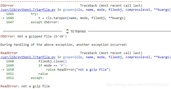
import tarfile

if not os.path.isdir('movie_data.csv'):
    with tarfile.open('movie_data.csv.gz', 'r:gz') as tar:
        tar.extractall()

ReadError: not a gzip file

import os
import gzip
import shutil
import pandas as pd

with gzip.open('movie_data.csv.gz', 'rb') as f_in, open ('movie_data.csv', 'wb') as f_out:
    shutil.copyfileobj(f_in, f_out)

##############################################

Solution : download the movie_data.csv.gz file then upzip it by using your tools(e.g. WinRAR or 7zip), upload to google drive

 

link = 'https://drive.google.com/file/d/17AYKouLCv7oOxloZ52COW0kEpVLRZikS/view?usp=sharing'
 
import pandas as pd 
  
# to get the id part of the file
# link.split("/")
# ['https:',
#  '',
#  'drive.google.com',
#  'file',
#  'd',
#  '17AYKouLCv7oOxloZ52COW0kEpVLRZikS',
#  'view?usp=sharing'] 
id = link.split("/")[-2] #==>'17AYKouLCv7oOxloZ52COW0kEpVLRZikS'
  
downloaded = drive.CreateFile({'id':id})  
downloaded.GetContentFile('movie_data.csv')   
  
df = pd.read_csv('movie_data.csv', encoding='utf-8') 
df.tail()

import tensorflow as tf

# Step 1: Create a dataset

target = df.pop('sentiment') #series # key: [value_list]
ds_raw = tf.data.Dataset.from_tensor_slices(
    (df.values, # array([ [...string...], [...string...], ...]
     target.values)
)# <TensorSliceDataset shapes: ((1,), ()), types: (tf.string, tf.int64)>

## inspection:
for item in ds_raw.take(3):
    # item[0].numpy() : array([...string...])
    tf.print( item[0].numpy()[0][:50], item[1] )

A -- An alternative way to get the dataset: using tensorflow_datasets

imdb_bldr = tfds.builder('imdb_reviews')
print(imdb_bldr.info)

imdb_bldr.download_and_prepare()

datasets = imdb_bldr.as_dataset(shuffle_files=False)

datasets.keys()

imdb_test = datasets['test']   # 25000,
imdb_train_valid = datasets['train'] # 25000,
    
# ## inspection:
for item in imdb_train_valid.take(1):
     tf.print( item )

 

prefetchDataset

imdb_test = datasets['test']   # 25000,
imdb_train_valid = datasets['train'] # 25000,

# tf.random.set_seed(1)

# ds_raw = imdb_train_valid.take(25000).shuffle(
#     25000, reshuffle_each_iteration=False
# ) # 25000 <== 0~24999

def transform_prefetchDataset(prefetchDataset):
    textList=[]
    labelList=[]
    for example in prefetchDataset:
        textList.append( example['text'].numpy() )
        labelList.append( example['label'].numpy() )
    textArr=np.array(textList)
    labelArr=np.array(labelList)
    
    return tf.data.Dataset.from_tensor_slices( ( textArr[..., np.newaxis],
                                                 labelArr
                                               ) )
ds_raw_train_valid = transform_prefetchDataset(imdb_train_valid)
ds_raw_test = transform_prefetchDataset(imdb_test)

ds_raw_train = ds_raw_train_valid.take(20000)
ds_raw_valid = ds_raw_train_valid.skip(20000)

# ## inspection:
for item in ds_raw_train.take(3):
     tf.print( item[0].numpy()[0][:50], item[1] )

###############################################

tf.random.set_seed(1)

ds_raw = ds_raw.shuffle(
    50000, reshuffle_each_iteration=False
) # 50000 <== 0~49999

ds_raw_test = ds_raw.take(25000)
ds_raw_train_valid = ds_raw.skip(25000)
ds_raw_train = ds_raw_train_valid.take(20000)
ds_raw_valid = ds_raw_train_valid.skip(20000)

# Step 2: find unique tokens  (words)

from collections import Counter
import tensorflow_datasets as tfds

token_counts = Counter()
tokenizer = tfds.features.text.Tokenizer() ##########################

for example in ds_raw_train:
    tokens = tokenizer.tokenize(example[0].numpy()[0])#numpy()[0] get first element in arr
    token_counts.update(tokens)

print('Vocab-size:', len(token_counts))

AttributeError: module 'tensorflow_datasets.core.features' has no attribute 'text'
###############################################
solutions: tokenizer = tfds.deprecated.text.Tokenizer()

tf.random.set_seed(1)

ds_raw = ds_raw.shuffle(
    50000, reshuffle_each_iteration=False
) # 50000 <== 0~49999

ds_raw_test = ds_raw.take(25000)
ds_raw_train_valid = ds_raw.skip(25000)
ds_raw_train = ds_raw_train_valid.take(20000)
ds_raw_valid = ds_raw_train_valid.skip(20000)

# Step 2: find unique tokens  (words)

from collections import Counter
import tensorflow_datasets as tfds

token_counts = Counter()
tokenizer = tfds.deprecated.text.Tokenizer()

for example in ds_raw_train:
    tokens = tokenizer.tokenize(example[0].numpy()[0])#numpy()[0] get first element in arr
    token_counts.update(tokens)

print('Vocab-size:', len(token_counts))

 is different with Vocab-size: 87007, since I take data from buffer twice.
solutions: re-run your code from  link = 'https://drive.google.com/file/d/17AYKouLCv7oOxloZ52COW0kEpVLRZikS/view?usp=sharing'

# Step 3: encoding each unique token into integers
######encoder = tfds.features.text.TokenTextEncoder( token_counts )
encoder = tfds.deprecated.text.TokenTextEncoder( token_counts )

# Step 3-A: define the function for transformation

# function will treat the input tensors as if the eager execution mode is enabled
def encode(text_tensor, label):
    text = text_tensor.numpy()[0]
    encoded_text = encoder.encode(text) # encoder = tfds.features.text.TokenTextEncoder( token_counts )
    return encoded_text, label

# Step 3-B: wrap the encode function to a TF Op that executes it eagerly
def encode_map_fn( text, label ):
    return tf.py_function( encode, inp=[text, label],
                                  Tout=(tf.int64, tf.int64))
    
ds_train = ds_raw_train.map( encode_map_fn ) # during mapping:  the eager execution will be disabled
ds_valid = ds_raw_valid.map( encode_map_fn ) # so wrap the encode function to a TF operator that executes it eagerly
ds_test = ds_raw_test.map( encode_map_fn )

tf.random.set_seed(1)
for example in ds_train.shuffle(1000).take(5):
    print('Sequence length:', example[0].shape)

example

# batching the datasets
train_data = ds_train.padded_batch(
    32, padded_shapes=([-1], # batch_size, here is 32
                       [])   # unset, all dimensions of all components are padded to the maximum size in the batch
)

valid_data = ds_valid.padded_batch(
    32, padded_shapes=([-1],
                       [])
)

test_data = ds_test.padded_batch(
    32, padded_shapes=([-1],
                       [])
)

from tensorflow.keras import Sequential
from tensorflow.keras.layers import Embedding
from tensorflow.keras.layers import SimpleRNN
from tensorflow.keras.layers import Dense

embedding_dim = 20
vocab_size = len( token_counts ) + 2 # Vocab-size: 87007

tf.random.set_seed(1)

# build the model
bi_lstm_model = tf.keras.Sequential([
    tf.keras.layers.Embedding(
        input_dim = vocab_size, # n+2
        output_dim = embedding_dim, #use a vector of length=embedding_dim to represent each word
        name = 'embed-layer'
    ),# Output Shape ==> (None_batch_size, None_each_input_length, output_dim=20)
    
    tf.keras.layers.Bidirectional(
        # lstm-layer:
        # return_sequences=False == many-to-one： (None_each_input_length, output_dim=64)==>(64)
        tf.keras.layers.LSTM(64, name='lstm-layer'),
        name = 'bidir-lstm', # default merge_mode='concat' ==> (64)==>(128) 
    ),# Output Shape ==> (None_batch_size, output_dim=128) 
    
    tf.keras.layers.Dense(64, activation='relu'),
    tf.keras.layers.Dense(1, activation='sigmoid')
])

bi_lstm_model.summary()

 

# compile and train:
bi_lstm_model.compile(
    optimizer = tf.keras.optimizers.Adam(1e-3),
    loss = tf.keras.losses.BinaryCrossentropy( from_logits=False),
    metrics=['accuracy']
)

history = bi_lstm_model.fit(
    train_data,
    validation_data = valid_data,
    epochs=10
)

# evaluate on the test data
test_results = bi_lstm_model.evaluate( test_data )
print( 'Test Acc.: {:.2f}%'.format(test_results[1]*100) )

 

     After training this model for 10 epochs, evaluation on the test data shows 82 percent accuracy. (Note that this result is not the best when compared to the state-of-the-art
methods used on the IMDb dataset. The goal was simply to show how RNN works.)

# if not os.path.exists('models'):
#     os.mkdir('models')
!mkdir models
    
bi_lstm_model.save('models/Birdir-LSTM-full-length-seq.h5')

from google.colab import drive
drive.mount('/content/gdrive')

 ==>==>
/content/gdrive/MyDrive/Colab Notebooks  # space between Colab Notebooks

!ls /content/gdrive/MyDrive/Colab\ Notebooks

 https://medium.com/@ml_kid/how-to-save-our-model-to-google-drive-and-reuse-it-2c1028058cb2

import os

if not os.path.exists('/content/gdrive/MyDrive/Colab Notebooks/models'):
    os.mkdir('/content/gdrive/MyDrive/Colab Notebooks/models')
# OR    
# !mkdir /content/gdrive/MyDrive/Colab\ Notebooks/models

bi_lstm_model.save('/content/gdrive/MyDrive/Colab Notebooks/models/Birdir-LSTM-full-length-seq.h5')

##################################################################

     We can also try other types of recurrent layers, such as SimpleRNN. However, as it turns out, a model built with regular recurrent layers won't be able to reach a good predictive performance (even on the training data). For example, if you try replacing the bidirectional LSTM layer in the previous code with a unidirectional SimpleRNN layer and train the model on full-length sequences, you may observe that the loss will not even decrease during training. The reason is that the sequences in this dataset are too long, so a model with a SimpleRNN layer cannot learn the long-term dependencies and may suffer from vanishing or exploding gradient problems.

     In order to obtain reasonable predictive performance on this dataset using a SimpleRNN, we can truncate the sequences. Also, utilizing our "domain knowledge," we may hypothesize that the last paragraphs of a movie review may contain most of the information about its sentiment. Hence, we can focus only on the last portion of each review. To do this, we will define a helper function, preprocess_datasets(), to combine the preprocessing steps 2-4. An optional argument to this function is max_seq_length, which determines how many tokens from each review should be used. For example, if we set max_seq_length=100 and a review has more than 100 tokens, only the last 100 tokens will be used. If max_seq_length is set to None, then full-length sequences will be used as before. Trying different values for max_seq_length will give us more insights on the capability of different RNN models to handle long sequences.

The code for the preprocess_datasets() function is as follows:

# ###  Step 1: Create a dataset
# target = df.pop('sentiment') #series # key: [value_list]
# ds_raw = tf.data.Dataset.from_tensor_slices(
#     (df.values, # array([ [...string...], [...string...], ...]
#      target.values) # without any column name
# )# <TensorSliceDataset shapes: ((1,), ()), types: (tf.string, tf.int64)>

# tf.random.set_seed(1)

# ds_raw = ds_raw.shuffle(
#     50000, reshuffle_each_iteration=False
# ) # 50000 <== 0~49999

# ds_raw_test = ds_raw.take(25000)
# ds_raw_train_valid = ds_raw.skip(25000)
# ds_raw_train = ds_raw_train_valid.take(20000)
# ds_raw_valid = ds_raw_train_valid.skip(20000)

from collections import Counter

def preprocess_datasets(
    ds_raw_train,
    ds_raw_valid,
    ds_raw_test,
    max_seq_length=None,
    batch_size=32 ):
  
  ######Step 1: (already done ==> creating a dataset)
  ######Step 2: find unique tokens in the training dataset
  tokenizer = tfds.deprecated.text.Tokenizer()
  token_counts = Counter()

  for example in ds_raw_train:# example[0] : [[review],...[review]]; example[1] : [sentiments]
    tokens = tokenizer.tokenize( example[0].numpy()[0])# numpy()[0] get first element in array
    if max_seq_length is not None:
      tokens = tokens[-max_seq_length:]
    token_counts.update(tokens)
  
  print( 'Vocab-size:', len(token_counts) )

  ######Step 3: encoding the texts(encoding each unique token into integers)
  encoder = tfds.deprecated.text.TokenTextEncoder( token_counts ) # use token from token_counts

  # Step 3-A: define the function for transformation
  # function will treat the input tensors as if the eager execution mode is enabled 
  def encode( text_tensor, label_tensor ): # A Python function which accepts a list of `Tensor` objects
    # need to call the numpy() method to get data from a tensor in the eager execution mode
    text = text_tensor.numpy()[0]
    encoded_text = encoder.encode(text) # return a integer list
    if max_seq_length is not None:
      encoded_text = encoded_text[-max_seq_length:] # an numpy array
    return encoded_text, label_tensor
    # Tout(tf.py_function): Specify the format of the numpy array returned by the encode method into tensor

  # Step 3-B: wrap the encode function to a TF Op that executes it eagerly
  # Why?
  # We use the map() method to transform each "text" in the 
  # dataset to a integer list ("encode action"). But, 
  # during transformations by the map() method, the eager execution will be disabled
  # tf.py_function to convert "encode method" into a TensorFlow operator ( that executes it eagerly )
  def encode_map_fn( text, label ):
    return tf.py_function( encode,
                           inp=[text, label], # inp: A list of Tensor objects
                           Tout=(tf.int64, tf.int64) # Tout: A list or tuple of tensorflow data types
                          )                                  # e.g. tf.tuple(tensors)
                          # Tout: Specify the format of the numpy array returned by the encode method into tensor
  
  ds_train = ds_raw_train.map( encode_map_fn )
  ds_valid = ds_raw_valid.map( encode_map_fn )
  ds_test = ds_raw_test.map( encode_map_fn )

  # step 4: batching the datasets
  train_data = ds_train.padded_batch(
      batch_size, padded_shapes=([-1], # batch_size
                                 []) # unset, all dimensions of all components are padded to the maximum size in the batch
  )
  valid_data = ds_valid.padded_batch(
      batch_size, padded_shapes=([-1], [])
  )
  test_data = ds_test.padded_batch(
      batch_size, padded_shapes=([-1], [])
  )

  return (train_data, valid_data, test_data, len(token_counts))

Next, we will define another helper function, build_rnn_model(), for building models with different architectures more conveniently:

from tensorflow.keras import Sequential
from tensorflow.keras.layers import Embedding
from tensorflow.keras.layers import SimpleRNN
from tensorflow.keras.layers import Dense

def build_rnn_model( embedding_dim, vocab_size,
                     recurrent_type='SimpleRNN',
                     n_recurrent_units = 64,
                     n_recurrent_layers = 1,
                     bidirectional=True ):
  tf.random.set_seed(1)
  
  # build the model
  model = tf.keras.Sequential()
  model.add( Embedding( input_dim=vocab_size, # n+2= len( token_counts ) + 2
                        output_dim = embedding_dim, # #use a vector with length=embedding_dim to represent each word
                        name='embed-layer')
  )

  for i in range(n_recurrent_layers):
    return_sequences = ( i < n_recurrent_layers-1 ) # return True OR False

    if recurrent_type == 'SimpleRNN':
      recurrent_layer = SimpleRNN( units=n_recurrent_units,
                                   return_sequences = return_sequences,
                                   name='simpRNN-layer-{}'.format(i) )
    elif recurrent_type == 'LSTM':
      recurrent_layer = LSTM( units=n_recurrent_units, 
                              return_sequences = return_sequences,
                              name='lstm-layer-{}'.format(i) )
    elif recurrent_type == 'GRU':
      recurrent_layer = GRU( units=n_recurrent_units,
                             return_sequences = return_sequences,
                             name='gru-layer-{}'.format(i) )
    if bidirectional:
      recurrent_layer = Bidirectional(
          recurrent_layer, name='bidir-'+recurrent_layer.name
      )
    model.add(recurrent_layer)

  model.add( tf.keras.layers.Dense(64, activation='relu') )
  model.add( tf.keras.layers.Dense(1, activation='sigmoid') )

  return model

     Now, using these two fairly general, but convenient, helper functions, we can readily compare different RNN models with different input sequence lengths. As an example, in the following code, we will try a model with a single recurrent layer of type SimpleRNN while truncating the sequences to a maximum length of 100 tokens:

from tensorflow.keras.layers import Bidirectional

batch_size = 32
embedding_dim = 20
max_seq_length = 100

train_data, valid_data, test_data, n = preprocess_datasets( ds_raw_train,ds_raw_valid, ds_raw_test,
                                                            max_seq_length=max_seq_length,
                                                            batch_size=batch_size
                                                          )
vocab_size=n+2

rnn_model = build_rnn_model(
                             embedding_dim, vocab_size,
                             recurrent_type = 'SimpleRNN',
                             n_recurrent_units=64,
                             n_recurrent_layers=1,
                             bidirectional=True
)

rnn_model.summary()

# loss = 'BinaryCrossentropy' since binary classification https://blog.csdn.net/Linli522362242/article/details/108414534

# Adam is better when the dataset is relatively sparse https://blog.csdn.net/Linli522362242/article/details/113311720
# some tokens may not exist in some reviews 
# e.g. while truncating the sequences to a maximum length of 100 tokens:

# loss = 'BinaryCrossentropy' since binary classification
# Adam is better when the dataset is relatively sparse
# some tokens may not exist in some reviews 
# e.g. while truncating the sequences to a maximum length of 100 tokens:
rnn_model.compile( optimizer=tf.keras.optimizers.Adam(1e-3),
                   loss=tf.keras.losses.BinaryCrossentropy( from_logits=False ),
                   metrics=['accuracy']
                 )
history = rnn_model.fit(
    train_data,
    validation_data = valid_data,
    epochs=10
)

results = rnn_model.evaluate( test_data )

print('Test Acc.: {:.2f}%'.format(results[1]*100))

     For instance, truncating the sequences to 100 tokens and using a bidirectional SimpleRNN layer resulted in 60 percent classification accuracy. Although the prediction is slightly lower when compared to the previous bidirectional LSTM model (82 percent accuracy on the test dataset), the performance on these truncated sequences is much better than the performance we could achieve with a SimpleRNN on full-length movie reviews. As an optional exercise, you can verify this by using the two helper functions we have already defined. Try it with max_seq_length=None and set the bidirectional argument inside the build_rnn_model() helper function to False. 

Uni-directional SimpleRNN with full-length sequences

from tensorflow.keras.layers import Bidirectional

batch_size = 32
embedding_dim = 20
max_seq_length = None ############

train_data, valid_data, test_data, n = preprocess_datasets( ds_raw_train,ds_raw_valid, ds_raw_test,
                                                            max_seq_length=max_seq_length,
                                                            batch_size=batch_size
                                                          )
vocab_size=n+2

rnn_model = build_rnn_model(
                             embedding_dim, vocab_size,
                             recurrent_type = 'SimpleRNN',
                             n_recurrent_units=64,
                             n_recurrent_layers=1,
                             bidirectional=False ############
)

rnn_model.summary()

# loss = 'BinaryCrossentropy' since binary classification
# Adam is better when the dataset is relatively sparse
# some tokens may not exist in some reviews 
# e.g. while truncating the sequences to a maximum length of 100 tokens:
rnn_model.compile( optimizer=tf.keras.optimizers.Adam(1e-3),
                   loss=tf.keras.losses.BinaryCrossentropy( from_logits=False ),
                   metrics=['accuracy']
                 )
history = rnn_model.fit(
    train_data,
    validation_data = valid_data,
    epochs=10
)

 

results = rnn_model.evaluate( test_data )
print('Test Acc.: {:.2f}%'.format(results[1]*100))

  

Project two – character-level language modeling in TensorFlow

     Language modeling is a fascinating application that enables machines to perform human language-related tasks, such as generating English sentences. One of the
interesting studies in this area is Generating Text with Recurrent Neural Networks, Ilya Sutskever, James Martens, and Geoffrey E. Hinton, Proceedings of the 28th International Conference on Machine Learning (ICML-11), 2011, https://pdfs.semanticscholar.org/93c2/0e38c85b69fc2d2eb314b3c1217913f7db11.pdf).

     In the model that we will build now, the input is a text document, and our goal is to develop a model that can generate new text that is similar in style to the input document. Examples of such an input are a book or a computer program in a specific programming language.

     In character-level language modeling, the input is broken down into a sequence of characters that are fed into our network one character at a time. The network will process each new character in conjunction with结合 the memory of the previously seen characters to predict the next one. The following figure shows an example of character-level language modeling (note that EOS stands for "end of sequence"):

     We can break this implementation down into three separate steps: preparing the data, building the RNN model, and performing next-character prediction and sampling to generate new text.

Preprocessing the dataset

In this section, we will prepare the data for character-level language modeling.

     To obtain the input data, visit the Project Gutenberg website at https://www.gutenberg.org/, which provides thousands of free e-books. For our example, you can download the book The Mysterious Island, by Jules Verne (published in 1874) in plain text format from http://www.gutenberg.org/files/1268/1268-0.txt.

     Note that this link will take you directly to the download page. If you are using macOS or a Linux operating system, you can download the file with the following command in the terminal:

! curl -O http://www.gutenberg.org/files/1268/1268-0.txt

 

###################################
https://curl.se/docs/manpage.html

     curl is a tool to transfer data from or to a server, using one of the supported protocols (DICT, FILE, FTP, FTPS, GOPHER, HTTP, HTTPS, IMAP, IMAPS, LDAP, LDAPS, MQTT, POP3, POP3S, RTMP, RTMPS, RTSP, SCP, SFTP, SMB, SMBS, SMTP, SMTPS, TELNET and TFTP). The command is designed to work without user interaction.

     curl offers a busload of useful tricks like proxy support, user authentication, FTP upload, HTTP post, SSL connections, cookies, file transfer resume, Metalink, and more. As you will see below, the number of features will make your head spin!

curl is powered by libcurl for all transfer-related features. See libcurl(3) for details.

OUTPUT

 

     If not told otherwise, curl writes the received data to stdout. It can be instructed to instead save that data into a local file, using the -o, --output or -O, --remote-name options. If curl is given multiple URLs to transfer on the command line, it similarly needs multiple options for where to save them.

     curl does not parse or otherwise "understand" the content it gets or writes as output. It does no encoding or decoding, unless explicitly asked so with dedicated command line options.
###################################

     If this resource becomes unavailable in the future, a copy of this text is also included in this chapter's code directory in the book's code repository at https://github.com/rasbt/python-machine-learning-book-3rd-edition/tree/master/ch16.

     Once we have downloaded the dataset, we can read it into a Python session as plain text. Using the following code, we will read the text directly from the downloaded
file and remove portions from the beginning and the end (these contain certain descriptions of the Gutenberg project). Then, we will create a Python variable, char_set, that represents the set of unique characters observed in this text:
... ...

... ...

... ...
The read() method returns the specified number of bytes from the file. Default is -1 which means the whole file.

import numpy as np

# Reading and processing text
with open('1268-0.txt', 'r') as fr:###########
    text = fr.read()

start_index = text.find('THE MYSTERIOUS ISLAND')
end_index = text.find('End of the Project Gutenberg')
print(start_index, end_index)

text = text[start_index:end_index]
char_set = set(text)
print('Total Length:', len(text))
print('Unique Characters:', len(char_set))

UnicodeDecodeError: 'charmap' codec can't decode byte 0x9d in position 817: character maps to <undefined>
Solution:

import numpy as np

# Reading and processing text
with open('1268-0.txt', 'r', encoding='utf-8') as fr:###########
    text = fr.read()

start_index = text.find('THE MYSTERIOUS ISLAND')
end_index = text.find('End of the Project Gutenberg')
print(start_index, end_index)

text = text[start_index:end_index]
char_set = set(text)
print('Total Length:', len(text))
print('Unique Characters:', len(char_set))

     After downloading and preprocessing the text, we have a sequence consisting of 1,112,350 characters in total and 80 unique characters. However, most NN libraries and RNN implementations cannot deal with input data in string format, which is why we have to convert the text into a numeric format. To do this, we will create a simple Python dictionary that maps each character to an integer, char2int. We will also need a reverse mapping to convert the results of our model back to text. Although the reverse can be done using a dictionary that associates integer keys with character values, using a NumPy array and indexing the array to map indices to those unique characters is more efficient. The following figure shows an example of converting characters into integers and the reverse for the words "Hello" and "world":

Building the dictionary to map characters to integers, and reverse mapping via indexing a NumPy array, as was shown in the previous figure, is as follows:

chars_sorted = sorted(char_set)
char2int = { ch:i for i,ch in enumerate(chars_sorted) }
char_array = np.array(chars_sorted) # convert set to np.array

text_encoded = np.array(
    [char2int[ch] for ch in text],
    dtype = np.int32
)

print('Text encoded shape: ', text_encoded.shape)

print( text[:15], '     == Encoding ==> ', text_encoded[:15] )
print( text_encoded[:15], ' == Reverse  ==> ', ''.join(char_array[text_encoded[:15]]) )
print( text_encoded[15:21], ' == Reverse  ==> ', ''.join(char_array[text_encoded[15:21]]) )

     The NumPy array text_encoded contains the encoded values for all the characters in the text. Now, we will create a TensorFlow dataset from this array:

import tensorflow as tf

ds_text_encoded = tf.data.Dataset.from_tensor_slices( text_encoded )
# ds_text_encoded # ==> <TensorSliceDataset shapes: (), types: tf.int32>

for ex in ds_text_encoded.take(5):
    print( '{} -> {}'.format(ex.numpy(), char_array[ex.numpy()]) )

     So far, we have created an iterable Dataset object for obtaining characters in the order they appear in the text. Now, let's step back and look at the big picture of what we are trying to do. For the text generation task, we can formulate the problem as a classification task.

Suppose we have a set of sequences of text characters that are incomplete, as shown in the following figure:

     In the previous figure, we can consider the sequences shown in the left-hand box to be the input. In order to generate new text, our goal is to design a model that
can predict the next character of a given input sequence, where the input sequence represents an incomplete text. For example, after seeing "Deep Learn", the model should predict "i" as the next character. Given that we have 80 unique characters, this problem becomes a multiclass classification task.

     Starting with a sequence of length 1 (that is, one single letter), we can iteratively generate new text based on this multiclass classification approach, as illustrated in
the following figure:

     To implement the text generation task in TensorFlow, let's first clip the sequence length to 40. This means that the input tensor, x, consists of 40 tokens. In practice, the sequence length impacts the quality of the generated text. Longer sequences can result in more meaningful sentences. For shorter sequences, however, the model might focus on capturing individual words correctly, while ignoring the context for the most part. Although longer sequences usually result in more meaningful sentences, as mentioned, for long sequences, the RNN model will have problems capturing long-term dependencies. Thus, in practice, finding a sweet spot最佳位置 and good value for the sequence length is a hyperparameter optimization problem, which we have to evaluate empirically[ɪm'pɪrɪklɪ]以经验为主地. Here, we are going to choose 40, as it offers a good tradeoff.

     As you can see in the previous figure, the inputs, x, and targets, y, are offset by one character. Hence, we will split the text into chunks of size 41: the first 40 characters will form the input sequence, x, and the last 40 elements will form the target sequence, y.

     We have already stored the entire encoded text in its original order in a Dataset object, ds_text_encoded. Using the techniques concerning transforming datasets that we already covered in this chapter (in the section Preparing the movie review data), can you think of a way to obtain the input, x, and target, y, as it was shown in the previous figure? The answer is very simple: we will first use the batch() method to create text chunks consisting of 41 characters each. This means that we will set batch_size=41. We will further get rid of the last batch if it is shorter than 41 characters. As a result, the new chunked dataset, named ds_chunks, will always contain sequences of size 41. The 41-character chunks will then be used to construct the sequence x (that is, the input), as well as the sequence y (that is, the target), both of which will have 40 elements. For instance, sequence x will consist of the elements with indices [0, 1, …, 39]. Furthermore, since sequence y will be shifted by one position with respect to x, its corresponding indices will be [1, 2, …, 40]. Then, we will apply a transformation function using the map() method to separate the x and y sequences accordingly:
#################################################

seq_length = 40
chunk_size = seq_length + 1
                                            # drop the last batch if it is shorter than chunk_size
ds_chunks = ds_text_encoded.batch(chunk_size, drop_remainder=True)

# inspection:
for seq in ds_chunks.take(1):# take 1 chunk with chunk_size = seq_length + 1
    input_seq = seq[:seq_length].numpy()
    target = seq[seq_length].numpy()
    print( input_seq, ' --> ', target )
    print( repr( ''.join(char_array[input_seq]) ),
           ' --> ', 
           repr( ''.join(char_array[target]) )
         )

why using repr()

# inspection:
for seq in ds_chunks.take(1):# take 1 chunk with chunk_size = seq_length + 1
    input_seq = seq[:seq_length].numpy()
    target = seq[seq_length].numpy()
    print( input_seq, ' --> ', target )
    print( ''.join(char_array[input_seq]),
           ' --> ', 
           ''.join(char_array[target])
         )

var = 'foo'

print(var)
print(repr(var))

Here, we assign a value 'foo' to var. Then, the repr() function returns "'foo'", 'foo' inside double-quotes. 

#################################################

seq_length = 40
chunk_size = seq_length + 1
                                            # drop the last batch if it is shorter than chunk_size
ds_chunks = ds_text_encoded.batch(chunk_size, drop_remainder=True)

# define the function for splitting x & y
def split_input_target( chunk ):
    input_seq = chunk[:-1]
    target_seq = chunk[1:]
    return input_seq, target_seq

ds_sequences = ds_chunks.map( split_input_target ) #[[input_seq, target_seq]...]

# inspection:
for eachChunk in ds_sequences.take(2):# take 2 chunks with chunk_size = seq_length + 1 each
    print(' Input (x):', repr( ''.join(char_array[ eachChunk[0].numpy() ])) )
    print('Target (y):', repr( ''.join(char_array[ eachChunk[1]])))
    print()

Let's take a look at some example sequences from this transformed dataset: 

     Finally, the last step in preparing the dataset is to divide this dataset into mini-batches. During the first preprocessing step to divide the dataset into batches, we created chunks of sentences. Each chunk represents one sentence, which corresponds to one training example. Now, we will shuffle the training examples and divide the inputs into mini-batches again; however, this time, each batch will contain multiple training examples:

# Batch size
BATCH_SIZE = 64
BUFFER_SIZE = 10000 # >>BATCH_SIZE*chunk_size=64*41=2624

tf.random.set_seed(1)
# ds_sequences : [[input_seq, target_seq]...[input_seq, target_seq]]
ds = ds_sequences.shuffle(BUFFER_SIZE).batch(BATCH_SIZE) # drop_remainder=True
ds

Building a character-level RNN model

     Now that the dataset is ready, building the model will be relatively straightforward. For code reusability, we will write a function, build_model, that defines an
RNN model using the Keras Sequential class. Then, we can specify the training parameters and call that function to obtain an RNN model:

def build_model( vocab_size, embedding_dim, rnn_units):
    model = tf.keras.Sequential([
        tf.keras.layers.Embedding(input_dim=vocab_size, # n without +2 since char_set = set(text)
                                  output_dim=embedding_dim ), #use a vector of length=embedding_dim to represent each character
        tf.keras.layers.LSTM(
            rnn_units, return_sequences=True),
        tf.keras.layers.Dense(vocab_size) # vocab_size <= charset_size = len(char_array)
    ])
    return model

charset_size = len(char_array)
embedding_dim = 256
rnn_units = 512

tf.random.set_seed(1)
model = build_model(
    vocab_size = charset_size,
    embedding_dim = embedding_dim,
    rnn_units=rnn_units
)
model.summary()

Notice that the LSTM layer in this model has the output shape (None, None, 512), which means the output of LSTM is rank 3. The first dimension stands for the number of batches, the second dimension for the output sequence length, and the last dimension corresponds to the number of hidden units. The reason for having rank-3 output from the LSTM layer is because we have specified return_sequences=True when defining our LSTM layer. A fully connected layer (Dense) receives the output from the LSTM cell and computes the logits for each element(character) of the output sequences. As a result, the final output of the model will be a rank-3 tensor as well.

     Furthermore, we specified activation=None for the final fully connected layer. The reason for this is that we will need to have the logits(logits =  ) as outputs of the model so that we can sample from the model predictions in order to generate new text. We will get to this sampling part later. For now, let's train the model:
# Adam is better when the dataset is relatively sparse https://blog.csdn.net/Linli522362242/article/details/113311720
# some tokens may not exist                                           # https://blog.csdn.net/Linli522362242/article/details/108414534

model.compile(
    optimizer = 'adam', # since the dataset is relatively sparse Sparse
    loss = tf.keras.losses.SparseCategoricalCrossentropy(
        from_logits=True
    )
)
model.fit(ds, epochs=20)

Save model in colab

from google.colab import drive
drive.mount('/content/gdrive')

# save both the model’s architecture (including every layer’s hyperparameters) 
# and the values of all the model parameters for every layer 
# (e.g., connection weights and biases).

# It also saves the optimizer (including its hyperparameters and any state it may have)


model.save('/content/gdrive/MyDrive/Colab Notebooks/models/LSTM_rnn_model.h5')

model = tf.keras.models.load_model("/content/gdrive/MyDrive/Colab Notebooks/models/LSTM_rnn_model.h5")

Now, we can evaluate the model to generate new text, starting with a given short string. In the next section, we will define a function to evaluate the trained model.

Evaluation phase – generating new text passages

     The RNN model we trained in the previous section returns the logits of size 80 for each unique character. These logits(logits =  ) can be readily converted to probabilities, via the softmax functionhttps://blog.csdn.net/Linli522362242/article/details/108414534, that a particular character will be encountered as the next character. To predict the next character in the sequence, we can simply select the element with the maximum logit value, which is equivalent to selecting the character with the highest probability. However, instead of always selecting the character with the highest likelihood, we want to (randomly) sample from the outputs; otherwise, the model will always produce the same text. TensorFlow already provides a function, tf.random.categorical(), which we can use to draw random samples from a categorical distribution.
To see how this works, let's generate some random samples from three categories [0, 1, 2], with input logits [1, 1, 1].
tf.math.softmax(logits).numpy()[0]

tf.random.set_seed(1)

logits = [[1.0, 1.0, 1.0]]
# or logits = tf.constant([ [1.0, 1.0, 1.0] ]) # hidden: auto-transform
print('Probabilities(softmax):', tf.math.softmax(logits).numpy()[0])
# np.exp(1.0) / ( np.exp(1.0) + np.exp(1.0) + np.exp(1.0) ) : 0.3333333333333333

samples = tf.random.categorical(
    logits=logits, num_samples=10
)
tf.print(samples.numpy())

tf.keras.activations.softmax(logits).numpy()[0] ==from ==> cp15_Classifying Images with Deep Convolutional NN_Loss_Cross Entropy_ax.text_mnist_ CelebA_Colab_ck_softmax https://blog.csdn.net/Linli522362242/article/details/108414534

tf.random.set_seed(1)

logits = tf.constant([ [1.0, 1.0, 1.0] ])
print( 'Probabilities(softmax):', tf.keras.activations.softmax(logits) )
print( 'Probabilities(softmax):', tf.keras.activations.softmax(logits).numpy()[0] )

samples = tf.random.categorical(
    logits=logits, num_samples=10
)
tf.print(samples.numpy())

     As you can see, with the given logits, the categories have the same probabilities (that is, equiprobable categories). Therefore, if we use a large sample size
(num_samples → ∞ ), we would expect the number of occurrences of each category to reach ≈ 1/3 of the sample size. If we change the logits to [1, 1, 3], then we would expect to observe more occurrences for category 2 (when a very large number of examples are drawn from this distribution):

tf.random.set_seed(1)

logits=[[1.0, 1.0, 3.0]] # hidden 3 categories
print( 'Probabilities(softmax):', tf.math.softmax(logits).numpy()[0] )

samples = tf.random.categorical(
    logits=logits, num_samples=10
)
tf.print(samples.numpy())

logits=tf.constant( [[1.0, 1.0, 3.0]] ) 
# logits.shape # ==> TensorShape([1, 3]) # 1x3=3 Note: after squeeze the result shape should be 3 as well
# tf.squeeze : Removes dimensions of size=1 from the shape of a tensor.
tf.shape( tf.squeeze(logits, axis=0) ) # ==> numpy=array( [1., 1., 3.] , dtype=float32) # remove 

     Using tf.random.categorical, we can generate examples based on the logits computed by our model ### scaled_logits = logits*scale_factor ###. We define a function, sample(), that receives a short starting string, starting_str, and generate a new string, generated_str, which is initially set to the input string(starting_str). Then, a string of size max_input_length is taken from the end of generated_str and encoded to a sequence of integers, encoded_input ### encoded_input = [ char2int[s] for s in starting_str ] ###. The encoded_input is passed to the RNN model to compute the logits ### logits = model( encoded_input ) ###. Note that the output from the RNN model is a sequence of logits with the same length as the input sequence, since we specified return_sequences=True for the last recurrent layer ### tf.keras.layers.LSTM( rnn_units, return_sequences=True) ### of our RNN model. Therefore, each element in the output of the RNN model represents the logits (here, a vector of size 80, which is the total number of characters) for the next character after observing the input sequence by the model ### e.g. the output logits: ( 10=encoded_input.shape[1]=len(input sequence) , 80 ).

#################################

tf.squeeze( new_char_indx ) : 
 ： 

     For shorter sequences, however, the model might focus on capturing individual words correctly, while ignoring the context for the most part.
only use the last element of the output logits:  Modify the following part of the code

    scaled_logits = logits*scale_factor # all elements * scale_factor

    new_char_indx = tf.random.categorical(
        scaled_logits[-1:,:], num_samples=1 #num_samples=1:only generate 1 random sample
    )#######################
    # print("new_char_indx shape: ", new_char_indx.shape) # (10++ until 40, num_samples=1)

    # new_char_indx[-1] : only use the "last element" of the output logits ~~ particular category/token in the vocab...
    # tf.squeeze : Removes dimensions of size=1 from the shape of the tensor "new_char_indx"
    #            ==>[...80...]
    new_char_indx = tf.squeeze( new_char_indx ).numpy() #######################

#################################

     Here, we only use the last elements (### [10++ until max_input_length=40,80] ###) of the output logits(that is,  , ), which is passed to the tf.random.categorical() function to generate a new sample(### num_samples=1 ### new_char_indx = tf.squeeze( new_char_indx )[-1].numpy() ###). This new sample is converted to a character (### str( char_array[new_char_indx] ) ###), which is then appended to the end of the generated string, generated_str, increasing its length by 1. Then, this process is repeated, taking the last max_input_length number of characters from the end of the generated_str, and using that to generate a new character until the length of the generated string reaches the desired value. The process of consuming the generated sequence as input for generating new elements is called auto-regression.

Returning sequences as output

     You may wonder why we use return_sequences=True when we only use the last character to sample a new character and ignore the rest of the output. While this question makes perfect sense, you should not forget that we used the entire output sequence for training. The loss is computed based on each prediction in the output and not just the last one.

The code for the sample() function is as follows:

# def build_model( vocab_size, embedding_dim, rnn_units):
#     model = tf.keras.Sequential([
#         tf.keras.layers.Embedding(input_dim=vocab_size, # n without +2 since char_set = set(text)
#                                   output_dim=embedding_dim ), #use a vector of length=embedding_dim to represent each word
#         tf.keras.layers.LSTM(
#             rnn_units, return_sequences=True),
#         tf.keras.layers.Dense(vocab_size)
#     ])
#     return model

# tf.random.set_seed(1)
# model = build_model(
#     vocab_size = charset_size,
#     embedding_dim = embedding_dim,
#     rnn_units=rnn_units
# )

# model.compile(
#     optimizer = 'adam',
#     loss = tf.keras.losses.SparseCategoricalCrossentropy(
#         from_logits=True
#     )
# )
# model.fit(ds, epochs=20)
def sample( model, starting_str, #  the input string
            len_generated_text=500,
            max_input_length=40,
            scale_factor=1.0 ):
  encoded_input = [ char2int[s] for s in starting_str ]
  encoded_input = tf.reshape(encoded_input, (1,-1) ) # one row multiple columns
  # print(encoded_input.shape) # ==> (1, len(starting_str)=10)

  generated_str = starting_str

  # Note that the methods predict, fit, train_on_batch, predict_classes, etc. 
  # will all update the states of the stateful layers in a model. This allows 
  # you to do not only stateful training, but also stateful prediction.

  # let's reset the states of the LSTM layer since we use an new sample to generate another new string
  model.reset_states() #  to reset the states of all layers in the model
 
  for i in range(len_generated_text): # model: prediction if activation is not none
    logits = model( encoded_input ) # based on encoded_input, get logit(p) = log( p/(1-p) )
    # tf.squeeze : Removes dimensions of size=1(here, only axis=0) from the shape of a tensor.
    # print( 'logits.shape:',logits.shape ) # (1,len(starting_str)=10++ until 40,80)
    logits = tf.squeeze( logits, 0 ) # ==> shape [10++ until 40,80] :[...[...80...]...]
    # until 40 since max_input_length=40
    
    scaled_logits = logits*scale_factor # all elements * scale_factor

    new_char_indx = tf.random.categorical(
        scaled_logits, num_samples=1 #num_samples=1:only generate 1 random sample
    )
    # print("new_char_indx shape: ", new_char_indx.shape) # (10++ until 40, num_samples=1)

    # new_char_indx[-1] : only use the "last element" of the output logits ~~ particular category/token in the vocab...
    # tf.squeeze : Removes dimensions of size=1 from the shape of the tensor "new_char_indx"
    #            ==>[...80...]
    new_char_indx = tf.squeeze( new_char_indx )[-1].numpy()
    
    generated_str += str( char_array[new_char_indx] )
    
    new_char_indx = tf.expand_dims( [new_char_indx], 0 )
    encoded_input = tf.concat(
        [encoded_input, new_char_indx], # axis=1
        axis=1 # since encoded_input shape [sample=1, sequences++] #[ [sequences++] ]
    )
    # print(encoded_input.shape) # (1, 10+1++until =41) # +1 since append an new_char_indx
    encoded_input = encoded_input[:, -max_input_length:] # get last max_input_length elements

  return generated_str

tf.random.set_seed(1)
print( sample(model, starting_str='The island') )

Let's now generate some new text: 

     As you can see, the model generates mostly correct words, and, in some cases, the sentences are partially meaningful. You can further tune the training parameters,
such as the length of input sequences for training, the model architecture, and sampling parameters (such as max_input_length).

     Furthermore, in order to control the predictability of the generated samples (that is, generating text following the learned patterns from the training text versus adding more randomness), the logits computed by the RNN model can be scaled before being passed to tf.random.categorical() for sampling. The scaling factor, 𝛼 , can be interpreted as the inverse of the temperature in physics. Higher temperatures result in more randomness versus more predictable behavior at lower temperatures. By scaling the logits with 𝛼 < 1 , the probabilities (logits =  ) computed by the softmax function become more uniform, as shown in the following code:

logits = np.array([ [1.0, 1.0, 3.0] ])

print( 'Probabilities before scaling:        ', tf.math.softmax(1.0*logits).numpy()[0] )
print( 'Probabilities after scaling with 0.5:', tf.math.softmax(0.5*logits).numpy()[0] )
print( 'Probabilities after scaling with 0.1:', tf.math.softmax(0.1*logits).numpy()[0] )

Smaller 𝛼 result in more randomness versus more predictable behavior at Larger 𝛼.

     As you can see, scaling the logits by 𝛼 = 0.1 results in near-uniform probabilities [0.31, 0.31, 0.38]. Now, we can compare the generated text with 𝛼 = 2.0 and 𝛼 = 0.5 , as shown in the following points:

• 𝛼 = 2.0 ➔ more predictable:

tf.random.set_seed(1)
print( sample(model, starting_str='The island', 
                     scale_factor=2.0) )

𝛼 = 0.5 ➔ more randomness:

tf.random.set_seed(1)
print( sample(model, starting_str='The island',
                     scale_factor=0.5) )

The results show that scaling the logits with 𝛼 = 0.5 (increasing the temperature) generates more random text. There is a tradeoff between the novelty[ˈnɑːvlti]新奇的 of the generated text and its correctness.

     In this section, we worked with character-level text generation, which is a sequence-tosequence (seq2seq) modeling task. While this example may not be very useful by itself, it is easy to think of several useful applications for these types of models; for example, a similar RNN model can be trained as a chatbot to assist users with simple queries.

Understanding language with the Transformer model

     We have solved two sequence modeling problems using RNN-based NNs. However, a new architecture has recently emerged that has been shown to outperform the RNN-based seq2seq models in several NLP tasks.

     It is called the Transformer architecture, capable of modeling global dependencies between input and output sequences, and was introduced in 2017 by Ashish
Vaswani, et. al., in the NeurIPS paper Attention Is All You Need (available online at http://papers.nips.cc/paper/7181-attention-is-all-you-need). The Transformer architecture is based on a concept called attention, and more specifically, the self-attention mechanism. Let's consider the sentiment analysis task that we covered earlier in this chapter. In this case, using the attention mechanism would mean that our model would be able to learn to focus on the parts of an input sequence that are more relevant to the sentiment.

Understanding the self-attention mechanism

     This section will explain the self-attention mechanism and how it helps a Transformer model to focus on important parts of a sequence for NLP(natural
language processing). The first subsection will cover a very basic form of self-attention to illustrate the overall idea behind learning text representations. Then, we will add different weight parameters so that we arrive at the self-attention mechanism that is commonly used in Transformer models.

A basic version of self-attention

     To introduce the basic idea behind self-attention, let's assume we have an input sequence of length T, , as well as an output sequence, . Each element of these sequences, and , are vectors of size d (that is, ∈ )
.e.g.
Then, for a seq2seq task, the goal of self-attention is to model the dependencies of each element in the output sequence to the input elements. In order to achieve this, attention mechanisms are composed of three stages.

1. Firstly, we derive importance weights based on the similarity between the current element and all other elements in the sequence.
2. Secondly, we normalize the weights, which usually involves the use of the already familiar softmax function.
3. Thirdly, we use these weights in combination with the corresponding sequence elements in order to compute the attention value.

     More formally, the output of self-attention is the weighted sum of all input sequences. For instance, for the ith input element, the corresponding output value
is computed as follows: 

     Here, the weights, , are computed based on the similarity between the current input element, , and all other elements in the input sequence. More concretely, this similarity is computed as the dot product between the current input element, , and another element in the input sequence, :
  e.g.==>==>

     After computing these similarity-based weights for the ith input and all inputs in the sequence ( to ) , the "raw" weights ( to ) are then normalized using the familiar softmax function, as follows: 
e.g. 

     Notice that as a consequence of applying the softmax function, the weights will sum to 1 after this normalization, that is, 

To recap, let's summarize the three main steps behind the self-attention operation:

1. 1. For a given input element, , and each jth element in the range [0, T], compute the dot product,

2. 2. Obtain the weight, , by normalizing the dot products using the softmax function
3. 3. Compute the output, , as the weighted sum over the entire input sequence:

These steps are further illustrated in the following figure: Self-Attention

Parameterizing the self-attention mechanism with query, key, and value weights

     Now that you have been introduced to the basic concept behind self-attention, this subsection summarizes the more advanced self-attention mechanism that is used in the Transformer model. Note that in the previous subsection, we didn't involve any learnable parameters when computing the outputs. Hence, if we want to learn a language model and want to change the attention values to optimize an objective, such as minimizing the classification error, we will need to change the word embeddings (that is, input vectors) that underlie each input element, (is a vector of size d).
###########https://towardsdatascience.com/illustrated-self-attention-2d627e33b20a
For this tutorial, we start with 3 input sequences, each with dimension d=4.

Input 1: [1, 0, 1, 0] 
Input 2: [0, 2, 0, 2]
Input 3: [1, 1, 1, 1]

###########
In other words, using the previously introduced basic self-attention mechanism, the Transformer model is rather limited with regard to how it can update or change the attention values during model optimization for a given sequence. To make the self-attention mechanism more flexible and amenable to model optimization, we will introduce three additional weight matrices that can be fit as model parameters during model training. We denote these three weight matrices as , , and  .They are used to project the inputs into query, key, and value sequence elements:

• Query sequence(Query representations): 
  e.g.
  Weights for query :

  [[1, 0, 1],
   [1, 0, 0],
   [0, 0, 1],
   [0, 1, 1]]

  Query representations

                 [1, 0, 1]
  [1, 0, 1, 0]   [1, 0, 0]   [1, 0, 2]
  [0, 2, 0, 2] x [0, 0, 1] = [2, 2, 2]
  [1, 1, 1, 1]   [0, 1, 1]   [2, 1, 3]

  
  
  #################################
• Key sequence (Key representation for Inputs) : 
  
  e.g.
  Weights for key :

[[0, 0, 1],
 [1, 1, 0],
 [0, 1, 0],
 [1, 1, 0]]

: 
X matmul U

               [0, 0, 1]
[1, 0, 1, 0]   [1, 1, 0]   [0, 1, 1]
[0, 2, 0, 2] x [0, 1, 0] = [4, 4, 0]
[1, 1, 1, 1]   [1, 1, 0]   [2, 3, 1]

#################################

• Value sequence: 
  e.g.
  Weights for value :

  [[0, 2, 0],
   [0, 3, 0],
   [1, 0, 3],
   [1, 1, 0]]

  Value representations for every input:

                 [0, 2, 0]
  [1, 0, 1, 0]   [0, 3, 0]   [1, 2, 3] 
  [0, 2, 0, 2] x [1, 0, 3] = [2, 8, 0]
  [1, 1, 1, 1]   [1, 1, 0]   [2, 6, 3]

  
   #################################
• Notes
  In practice, a bias vector may be added to the product of matrix multiplication.

      Here, both and are vectors of size . Therefore, the projection matrices and have the shape , while has the shape . For simplicity, we can design these vectors to have the same shape, for example, using  . Now, instead of computing the unnormalized weight as the pairwise dot product between the given input sequence element, , and the jth sequence element, ,
we can compute the dot product between the query and key: 
e.g.
     Step 4: Calculate attention scores for Input1(Notice that we only use the query from Input 1. Later we’ll work on repeating this same step for the other querys.)

            [0, 4, 2]
[1, 0, 2] x [1, 4, 3] = [2, 4, 4]
            [1, 0, 1]

################################

We can then further use m, or, more precisely, , to scale before normalizing it via the softmax function, as follows: 
Note that scaling by will ensure that the Euclidean length of the weight vectors will be approximately in the same range.
e.g.
Step 5: Calculate softmax

softmax([2, 4, 4]) = [0.0, 0.5, 0.5]

 Note that we round of to 1 decimal place here for readability.
################################
Step 6: Multiply scores with values

1: 0.0 * [1, 2, 3] = [0.0, 0.0, 0.0]
2: 0.5 * [2, 8, 0] = [1.0, 4.0, 0.0]
3: 0.5 * [2, 6, 3] = [1.0, 3.0, 1.5]

Step 7: Sum weighted values to get Output 1

  [0.0, 0.0, 0.0]
+ [1.0, 4.0, 0.0]
+ [1.0, 3.0, 1.5]
-----------------
= [2.0, 7.0, 1.5]

Step 8: Repeat for Input 2 & Input 3

Now that we’re done with Output 1, we repeat Steps 4 to 7 for Output 2 and Output 3. I trust that I can leave you to work out the operations yourself 

output matrix Z shape : number fo sequences(here is 3 inputs) x m(For simplicity,=3)

################################https://towardsdatascience.com/illustrated-self-attention-2d627e33b20a
https://www.cnblogs.com/USTC-ZCC/p/11155636.html
http://jalammar.github.io/illustrated-transformer/

Multi-head attention and the Transformer block

     Another trick that greatly improves the discriminatory [dɪˈskrɪmɪnətɔri]歧视的 power of the self-attention mechanism is multi-head attention (MHA), which combines multiple self-attention operations together. In this case, each self-attention mechanism is called a head, which can be computed in parallel. Using r parallel heads, each head results in a vector, h, of size m. These vectors are then concatenated to obtain a vector, z, with the shape 𝑟 × 𝑚 . Finally, the concatenated vector is projected using ( an additional ) the output matrix to obtain the final output, as follows:

##################http://jalammar.github.io/illustrated-transformer/
If we do the same self-attention calculation we outlined above, just r=8 different times with different weight matrices, we end up with r=8 different Z matrices( Each Z shape: 2 inputs x m (here, For simplicity,=3) 

##################http://jalammar.github.io/illustrated-transformer/
The architecture of a Transformer block is shown in the following figure:

    Notice that in the Transformer architecture shown in the previous figure, we added two additional components that we haven't discussed yet. One of these components is the residual connection, which adds the output from a layer (or even a group of layers) to its input, that is, x + layer(x). The block consisting of a layer (or multiple layers) with such a residual connection is called a residual block. The Transformer block shown in the previous figure has two residual blocks.

     The other new component is layer normalization, which is denoted in the previous figure as "Layer norm." There is a family of normalization layers including batch
normalization, which we will cover in Chapter 17, Generative Adversarial Networks for Synthesizing New Data. For now, you can think of layer normalization as a fancy or
more advanced way of normalizing or scaling the NN inputs and activations in each layer.

     Returning to the illustration of the Transformer model in the previous figure, let's now discuss how this model works.

• First, the input sequence is passed to the MHA layers, which is based on the self-attention mechanism that we discussed earlier.
   
• In addition, the input sequences are added to the output of the MHA layers via the residual connections—this ensures that the earlier layers will receive sufficient gradient signals during training, which is a common trick that is used to improve training speed and convergence. If you are interested, you can read more about the concept behind residual connections in the research article Deep Residual Learning for Image Recognition, by Kaiming He, Xiangyu Zhang, Shaoqing Ren, and Jian Sun, which is freely available at https://openaccess.thecvf.com/content_cvpr_2016/html/He_Deep_Residual_Learning_CVPR_2016_paper.html.
   
• After the input sequences are added to the output of the MHA layers, the outputs(from the residual block) are normalized via layer normalization. These normalized signals then go through a series of MLP (that is, fully connected) layers, which also have a residual connection.
   
• Finally, the output from the residual block is normalized again and returned as the output sequence, which can be used for sequence classification or sequence generation.

     Instructions for implementing and training Transformer models were omitted to conserve space. However, the interested reader can find an excellent implementation and walk-through in the official TensorFlow documentation at https://www.tensorflow.org/tutorials/text/transformer.

Summary

     In this chapter, you first learned about the properties of sequences that make them different to other types of data, such as structured data or images. We then
covered the foundations of RNNs for sequence modeling. You learned how a basic RNN model works and discussed its limitations with regard to capturing longterm
dependencies in sequence data. Next, we covered LSTM cells, which consist of a gating mechanism to reduce the effect of exploding and vanishing gradient
problems, which are common in basic RNN models.

     After discussing the main concepts behind RNNs, we implemented several RNN models with different recurrent layers using the Keras API. In particular, we
implemented an RNN model for sentiment analysis, as well as an RNN model for generating text. Finally, we covered the Transformer model, which leverages
the self-attention mechanism in order to focus on the relevant parts of a sequence.

     In the next chapter, you will learn about generative models and, in particular, generative adversarial networks (GANs), which have shown remarkable results
in the computer vision community for various vision tasks.