


In the https://blog.csdn.net/Linli522362242/article/details/113846940, we focused on recurrent neural networks for modeling sequences. In this chapter, we will explore generative adversarial networks (GANs) and see their application in synthesizing new data samples. GANs are considered to be the most important breakthrough in deep learning, allowing computers to generate new data (such as new images).
we will cover the following topics:
- • Introducing generative models for synthesizing new data
- • Autoencoders, variational autoencoders (VAEs), and their relationship to GANs
- • Understanding the building blocks of GANs
- • Implementing a simple GAN model to generate handwritten digits
- • Understanding transposed convolution and batch normalization (BatchNorm or BN)
- • Improving GANs: deep convolutional GANs and GANs using the Wasserstein distance
Introducing generative adversarial networks
Let's first look at the foundations of GAN models. The overall objective of a GAN is to synthesize new data that has the same distribution as its training dataset. Therefore, GANs, in their original form, are considered to be in the unsupervised learning category of machine learning tasks, since no labeled data is required. It is worth noting, however, that extensions made to the original GAN can lie in both semi-supervised and supervised tasks.
The general GAN concept was first proposed in 2014 by Ian Goodfellow and his colleagues as a method for synthesizing new images using deep neural networks (NNs) (Goodfellow, I., Pouget-Abadie, J., Mirza, M., Xu, B., Warde-Farley, D., Ozair, S., Courville, A. and Bengio, Y., Generative Adversarial Nets, in Advances in Neural Information Processing Systems, pp. 2672-2680, 2014). While the initial GAN architecture proposed in this paper was based on fully connected layers, similar to multilayer perceptron architectures, and trained to generate low-resolution MNISTlike handwritten digits, it served more as a proof of concept to demonstrate the feasibility可行性 of this new approach.
However, since its introduction, the original authors, as well as many other researchers, have proposed numerous improvements and various applications in different fields of engineering and science; for example, in computer vision, GANs are used for image-to-image translation (learning how to map an input image to an output image), image super-resolution (making a high-resolution image from a low-resolution version), image inpainting图像修复 (learning how to reconstruct the missing parts of an image), and many more applications. For instance, recent advances in GAN research have led to models that are able to generate new, high-resolution face images. Examples of such high-resolution images can be found on https://www.thispersondoesnotexist.com/, which showcases synthetic face images generated by a GAN.
Starting with autoencoders
Before we discuss how GANs work, we will first start with autoencoders, which can compress and decompress training data. While standard autoencoders cannot generate new data, understanding their function will help you to navigate GANs in the next section.
Autoencoders are composed of two networks concatenated together: an encoder network(or recognition network) and a decoder network(or generative network). The encoder network receives a d-dimensional input feature vector associated with example x (that is, 𝒙 ∈ ![]() ) and encodes it into a p-dimensional vector, z (that is, 𝒛 ∈
) and encodes it into a p-dimensional vector, z (that is, 𝒛 ∈ ![]() ). In other words, the role of the encoder is to learn how to model the function 𝒛 = 𝑓(𝒙) . The encoded vector, z, is also called the latent vector, or the latent feature representation. Typically, the dimensionality of the latent vector is less than that of the input examples; in other words, p < d. Hence, we can say that the encoder acts as a data compression function. Then, the decoder decompresses 𝒙̂ from the lower-dimensional latent vector, z, where we can think of the decoder as a function,𝒙̂ = 𝑔(𝒛). A simple autoencoder architecture is shown in the following figure, where the encoder and decoder parts consist of only one fully connected layer each:
). In other words, the role of the encoder is to learn how to model the function 𝒛 = 𝑓(𝒙) . The encoded vector, z, is also called the latent vector, or the latent feature representation. Typically, the dimensionality of the latent vector is less than that of the input examples; in other words, p < d. Hence, we can say that the encoder acts as a data compression function. Then, the decoder decompresses 𝒙̂ from the lower-dimensional latent vector, z, where we can think of the decoder as a function,𝒙̂ = 𝑔(𝒛). A simple autoencoder architecture is shown in the following figure, where the encoder and decoder parts consist of only one fully connected layer each: vs
vs  https://blog.csdn.net/Linli522362242/article/details/116576478
###################################
The connection between autoencoders and dimensionality reduction
In Chapter 5, Compressing Data via Dimensionality Reduction https://blog.csdn.net/Linli522362242/article/details/105196037, you learned about dimensionality reduction techniques, such as principal component analysis (PCA, Principal Component Analysis (PCA)主成分分析 is by far the most popular dimensionality reduction algorithm. First it identifies the hyperplane that lies closest to the data, and then it projects the data onto it.) and linear discriminant analysis (LDA). Autoencoders can be used as a dimensionality reduction technique as well. In fact, when there is no nonlinearity in either of the two subnetworks (encoder and decoder), then the autoencoder approach is almost identical to PCA.
In this case, if we assume the weights of a single-layer encoder (no hidden layer and no nonlinear activation function
##################### https://blog.csdn.net/Linli522362242/article/details/116065910
encoder.trainable_variables
# vocab_inp_size = len( inp_lang_tokenizer.word_index )+1 #==>9693=9692 words + 1 oov
# GRU( units =1024 )
![]() and
and 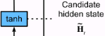
https://blog.csdn.net/Linli522362242/article/details/114941730
# tf.Variable encoder.trainable_variables:
encoder/embedding/embeddings : shape=(input_dim=vocab_size==9693, # 9692 words + 1 oov
output_dim=embedding_dim==256)
encoder/gru/gru_cell/kernel for input : shape=(256=embedding_dim, 3072=W_x_reset(256, 1024 hidden units)+
W_x_update(256, 1024 hidden units)+
W_x_candidate(256, 1024 hidden units))
for recurrent stateencoder/gru/gru_cell/recurrent_kernel : shape=(1024 hidden units, 3072=W_h_reset(1024 hidden units, 1024 hidden units)+
W_h_update(1024 hidden units, 1024 hidden units)+
W_h_candidate(1024 hidden units, 1024 hidden units))
encoder/gru/gru_cell/bias : shape=(2 kernel ==>just 1 kernel, 3072=reset gate bias(1x1024 hidden units) +
update gate bias(1x1024 hidden units) +
candidate hidden state bias(1x1024 hidden units) )
#####################
) are denoted by the matrix U, then the encoder models 𝒛 = ![]() (VS Equation 8-2. Projecting the training set down to d dimensions
(VS Equation 8-2. Projecting the training set down to d dimensions![]() https://blog.csdn.net/Linli522362242/article/details/105139547). Similarly, a single-layer linear decoder models 𝒙̂ = 𝑼𝒛 (VS Equation 8-3. PCA inverse transformation, back to the original number of dimensions
https://blog.csdn.net/Linli522362242/article/details/105139547). Similarly, a single-layer linear decoder models 𝒙̂ = 𝑼𝒛 (VS Equation 8-3. PCA inverse transformation, back to the original number of dimensions ![]() ). Putting these two components together, we have 𝒙̂ =
). Putting these two components together, we have 𝒙̂ = ![]() . This is exactly what PCA does, with the exception that PCA has an additional orthonormal正交的 constraint:
. This is exactly what PCA does, with the exception that PCA has an additional orthonormal正交的 constraint: ![]() .
.
###################################
While the previous figure depicts an autoencoder without hidden layers within the encoder and decoder, we can, of course, add multiple hidden layers with nonlinearities (as in a multilayer NN) to construct a deep autoencoder that can learn more effective data compression and reconstruction functions. Also, note that the autoencoder mentioned in this section uses fully connected layers. When we work with images, however, we can replace the fully connected layers with convolutional layers, as you learned in Cp15, Classifying Images with Deep Convolutional Neural Networks https://blog.csdn.net/Linli522362242/article/details/108414534.
a fully connected layer, or a dense layer
When all the neurons in a layer are connected to every neuron in the previous layer (i.e., its input neurons), the layer is called a fully connected layer, or a dense layer.
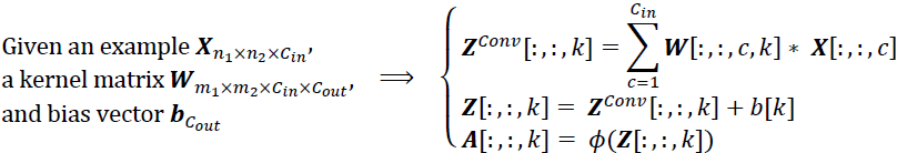
Equation 10-2. Computing the outputs of a fully connected layer : ![]()
In this equation:https://blog.csdn.net/Linli522362242/article/details/106433059
- As always, X represents the matrix of input features. It has one row per instance and one column per feature.
- The weight matrix W contains all the connection weights except for the ones from the bias neuron. It has one row per input neuron and one column per artificial neuron in the layer.
- The bias vector b contains all the connection weights between the bias neuron and the artificial neurons. It has one bias term per artificial neuron.
- The function ϕ is called the activation function: when the artificial neurons are TLUs, it is a step function (but we will discuss other activation functions shortly).
- W X_i b
- the dense layer’s output was a tensor of shape [batch size, 10] https://blog.csdn.net/Linli522362242/article/details/108669444
# Implementing a CNN in TensorFlow low-level API by using tensorflow.compat.v1 import tensorflow.compat.v1 as tf import numpy as np def fc_layer(input_tensor, # Tensor("Placeholder:0", shape=(None, 7, 7, 4), dtype=float32) name, # name='fctest' n_output_units, # n_output_units=10 activation_fn=None):# activation_fn=tf.nn.relu with tf.variable_scope(name): input_shape = input_tensor.get_shape().as_list()[1:] # return [7, 7, 4] n_input_units = np.prod(input_shape) # return 196 = 7*7*4 = n_1*n_2*input_channel if len(input_shape) > 1: input_tensor = tf.reshape(input_tensor, shape=(-1, n_input_units) )#Tensor("fctest/Reshape:0", shape=(None,196), dtype=float32) # n_output_units =1x1x10 weights_shape = [n_input_units, n_output_units] #[196, 10] weights = tf.get_variable(name='_weights', shape=weights_shape) print(weights) # <tf.Variable 'fctest/_weights:0' shape=(196, 10) dtype=float32> biases = tf.get_variable(name='_biases', initializer=tf.zeros( shape=[n_output_units] ) ) print(biases) # <tf.Variable 'fctest/_biases:0' shape=(10,) dtype=float32> # mat_shape(batches, 196) x mat_shape(196, 10) ==> mat_shape(batches, 10) layer = tf.matmul(input_tensor, weights)#shape(None, 10) print(layer) # Tensor("fctest/MatMul:0", shape=(None, 10), dtype=float32) layer = tf.nn.bias_add(layer, biases, name='net_pre-activation') print(layer) # Tensor("fctest/net_pre-activation:0", shape=(None, 10), dtype=float32) if activation_fn is None: return layer layer = activation_fn(layer, name='activation') print(layer) # Tensor("fctest/activation:0", shape=(None, 10), dtype=float32) return layer ## testing: g = tf.Graph() with g.as_default(): x = tf.placeholder(tf.float32, shape=[None, 7, 7, 4]) fc_layer(x, name='fctest', n_output_units=10, activation_fn=tf.nn.relu) del g, x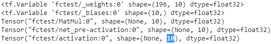 7*7*4channels=196
FCN(Fully Convolutional Networks)
 and
and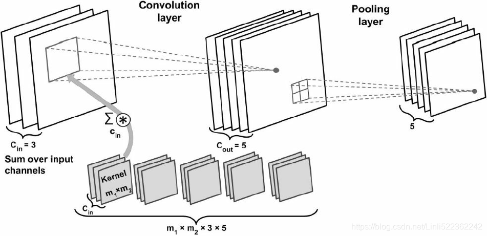
To convert a dense layer to a convolutional layer,
- the number of filters
 in the convolutional layer must be equal to the number of units in the dense layer,
 - the filter size(OR kernel size, weight matrix W ) must be equal to the size of the input feature maps,
- and you must use "valid" padding.
- The stride may be set to 1 or more, as we will see shortly.
- the convolutional layer will output a tensor of shape [batch size, 1, 1, 10]https://blog.csdn.net/Linli522362242/article/details/108669444
# Implementing a CNN in TensorFlow low-level API by using tensorflow.compat.v1 import tensorflow.compat.v1 as tf import numpy as np ## wrapper functions def conv_layer(input_tensor, # Tensor("Placeholder:0", shape=(None, 7, 7, 4), dtype=float32) name, # name='convtest' kernel_size, # kernel_size=(7, 7) n_output_channels, # n_output_channels=10 padding_mode='VALID', strides=(1, 1, 1, 1)): with tf.variable_scope(name):# convtest/ ## get n_input_channels: ## input tensor shape: ## [batch x width x height x channels_in] input_shape = input_tensor.get_shape().as_list() #return [None, 7, 7, 4] n_input_channels = input_shape[-1] # [ width, height, C_in, C_out ] weights_shape = (list(kernel_size) + [n_input_channels, n_output_channels]) weights = tf.get_variable(name='_weights', shape=weights_shape) print(weights) #<tf.Variable 'convtest/_weights:0' shape=(7, 7, 4, 10) dtype=float32> ################################################ conv = tf.nn.conv2d(input=input_tensor, filter=weights, strides=strides, padding=padding_mode) #padding_mode='VALID' ==>p=0 print(conv) #Tensor("convtest/Conv2D:0", shape=(None, 1, 1, 10), dtype=float32) # output shape 1 = (7 + 2*0 - 7)/1 +1=1 ################################################ biases = tf.get_variable(name='_biases', initializer=tf.zeros( shape=[n_output_channels] ) ) print(biases) #<tf.Variable 'convtest/_biases:0' shape=(10,) dtype=float32> conv = tf.nn.bias_add(conv, biases, name='net_pre-activation') print(conv)#Tensor("convtest/net_pre-activation:0", shape=(None,1,1,10), dtype=float32) ################################################# conv = tf.nn.relu(conv, name='activation') print(conv)# Tensor("convtest/activation:0", shape=(None, 1, 1, 10), dtype=float32) return conv ## testing g = tf.Graph() with g.as_default(): x = tf.placeholder(tf.float32, shape=[None, 7, 7, 4]) conv_layer(x, name='convtest', kernel_size=(7, 7), n_output_channels=10) del g, x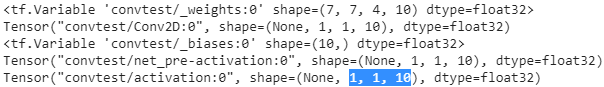 ...
...
How many trainable parameters exist in the preceding figure?
To illustrate the advantages of convolution, parameter-sharing and sparse connectivity, let's work through an example. The convolutional layer in the network shown in the preceding figure is a four-dimensional tensor. So, there are 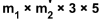 parameters associated with the kernel. Furthermore, there is a bias vector for each output feature map of the convolutional layer. Thus, the size of the bias vector is 5
  . Pooling layers do not have any (trainable) parameters; therefore, we can write the following: https://blog.csdn.net/Linli522362242/article/details/114817809
![]() (+5 since the bias vector) OR kernel[width, height, c_in, c_out] + bias[c_out]
(+5 since the bias vector) OR kernel[width, height, c_in, c_out] + bias[c_out]
If input tensor is of size ![]() , assuming that the convolution is performed with mode='same', then the output feature maps would be of size
, assuming that the convolution is performed with mode='same', then the output feature maps would be of size ![]() .
.
Note that this number ![]() is much smaller than the case if we wanted to have a fully connected layer instead of the convolution layer. In the case of a fully connected layer, the number of parameters for the weight matrix to reach the same number of output units would have been as follows:
is much smaller than the case if we wanted to have a fully connected layer instead of the convolution layer. In the case of a fully connected layer, the number of parameters for the weight matrix to reach the same number of output units would have been as follows:
![]() OR n_input_units(= n_1*n_2*input_channel) x n_output_units(=n_1*n_2*output_channel, in my code is 10=1*1*10 and use mode='valid')
OR n_input_units(= n_1*n_2*input_channel) x n_output_units(=n_1*n_2*output_channel, in my code is 10=1*1*10 and use mode='valid')
In addition, the size of the bias vector is n_output_units= ![]() (one bias element for each output unit). Given that
(one bias element for each output unit). Given that ![]() and
and ![]() , we can see that the difference in the number of trainable parameters is huge.
, we can see that the difference in the number of trainable parameters is huge.
#################################################
Other types of autoencoders based on the size of latent space
As previously mentioned, the dimensionality of an autoencoder's latent space is typically lower than the dimensionality of the inputs (p < d), which makes autoencoders suitable for dimensionality reduction. For this reason, the latent vector is also often referred to as the "bottleneck," and this particular configuration of an autoencoder is also called undercomplete不完整(It is forced to learn the most important features in the input data (and drop the unimportant ones)). However, there is a different category of autoencoders, called overcomplete, where the dimensionality of the latent vector, z, is, in fact, greater than the dimensionality of the input examples (p > d).
When training an overcomplete autoencoder, there is a trivial solution where the encoder and the decoder can simply learn to copy (memorize) the input features to their output layer. Obviously, this solution is not very useful. However, with some modifications to the training procedure, overcomplete autoencoders can be used for noise reduction.
In this case,
- during training, random noise, 𝝐 , is added to the input examples and the network learns to reconstruct the clean example, x, from the noisy signal, 𝒙 + 𝝐 . Then,
- at evaluation time, we provide the new examples that are naturally noisy (that is, noise is already present such that no additional artificial noise, 𝝐 , is added) in order to remove the existing noise from these examples. This particular autoencoder architecture and training method is referred to as a denoising autoencoder.
If you are interested, you can learn more about it in the research article Stacked denoising autoencoders: Learning useful representations in a deep network with a local denoising criterion by Vincent et al., which is freely available at https://www.jmlr.org/papers/v11/vincent10a.html.
 Figure 17-8. Denoising autoencoders, with Gaussian noise (left) or dropout (right)https://blog.csdn.net/Linli522362242/article/details/116576478
#################################################
Generative models for synthesizing new data
Autoencoders are deterministic models, which means that after an autoencoder is trained, given an input, x, it will be able to reconstruct the input from its compressed version in a lower-dimensional space![]() . Therefore, it cannot generate new data beyond reconstructing its input through the transformation of the compressed representation.
. Therefore, it cannot generate new data beyond reconstructing its input through the transformation of the compressed representation.
A generative model, on the other hand, can generate a new example, 𝒙̃ , from a random vector, z (corresponding to the latent representation, 𝒛 = 𝑓(𝒙)). A schematic representation of a generative model is shown in the following figure. The random vector, z, comes from a simple distribution with fully known characteristics, so we can easily sample from such a distribution. For example, each element of z may come from the uniform distribution in the range [–1, 1] (for which we write ![]() or from a standard normal distribution (in which case, we write
or from a standard normal distribution (in which case, we write ![]() ).
).
As we have shifted our attention from autoencoders to generative models, you may have noticed that the decoder component of an autoencoder has some similarities with a generative model. In particular, they both receive a latent vector, z, as input and return an output in the same space as x. (For the autoencoder, 𝒙̂ is the reconstruction of an input, x, and for the generative model, 𝒙̃ is a synthesized合成的 sample.)
However, the major difference between the two is that we do not know the distribution of z in the autoencoder, while in a generative model, the distribution of z is fully characterizable. It is possible to generalize an autoencoder into a generative model, though. One approach is VAEs(variational autoencoders).
 Figure 17-12. Variational autoencoder (left) and an instance going through it (right) https://blog.csdn.net/Linli522362242/article/details/116576478
In a VAE receiving an input example, x, the encoder network is modified in such a way that it computes two moments of the distribution of the latent vector: the mean, 𝝁, and variance, ![]() . During the training of a VAE, the network is forced to match these moments with those of a standard normal distribution (that is, zero mean and unit variance). Then, after the VAE model is trained, the encoder is discarded, and we can use the decoder network to generate new examples, 𝒙̃ , by feeding random z vectors from the "learned" Gaussian distribution.
. During the training of a VAE, the network is forced to match these moments with those of a standard normal distribution (that is, zero mean and unit variance). Then, after the VAE model is trained, the encoder is discarded, and we can use the decoder network to generate new examples, 𝒙̃ , by feeding random z vectors from the "learned" Gaussian distribution.
Besides VAEs, there are other types of generative models, for example, autoregressive models and normalizing flow models. However, in this chapter, we are only going to focus on GAN models, which are among the most recent and most popular types of generative models in deep learning.
What is a generative model?
Note that generative models are traditionally defined as algorithms that model data input distributions, p(x), or the joint distributions of the input data and associated targets, p(x, y). By definition, these models are also capable of sampling from some feature, ![]() , conditioned on another feature,
, conditioned on another feature, ![]() , which is known as conditional inference. In the context of deep learning, however, the term generative model is typically used to refer to models that generate realistic-looking data生成逼真的数据. This means that we can sample from input distributions, p(x), but we are not necessarily able to perform conditional inference但是我们不一定能够执行条件推断。.
, which is known as conditional inference. In the context of deep learning, however, the term generative model is typically used to refer to models that generate realistic-looking data生成逼真的数据. This means that we can sample from input distributions, p(x), but we are not necessarily able to perform conditional inference但是我们不一定能够执行条件推断。.
Generating new samples with GANs
To understand what GANs do in a nutshell, let's first assume we have a network that receives a random vector, z, sampled from a known distribution and generates an output image, x. We will call this network generator (G) and use the notation 𝒙̃ = 𝐺(𝒛) to refer to the generated output. Assume our goal is to generate some images, for example, face images, images of buildings, images of animals, or even handwritten digits such as MNIST.
As always, we will initialize this network with random weights. Therefore, the first output images, before these weights are adjusted, will look like white noise. Now, imagine there is a function that can assess评估 the quality of images (let's call it an assessor function).
If such a function exists, we can use the feedback from that function(assessor function) to tell our generator network how to adjust its weights in order to improve the quality of the generated images. This way, we can train the generator based on the feedback from that assessor function, such that the generator learns to improve its output toward producing realistic-looking逼真的 images.
While an assessor function, as described in the previous paragraph, would make the image generation task very easy, the question is whether such a universal function to assess the quality of images exists and, if so, how it is defined. Obviously, as humans, we can easily assess the quality of output images when we observe the outputs of the network; although, we cannot (yet) backpropagate the result from our brain to the network. Now, if our brain can assess the quality of synthesized images, can we design an NN model to do the same thing? In fact, that's the general idea of a GAN. As shown in the following figure, a GAN model consists of an additional NN called discriminator (D), which is a classifier that learns to detect a synthesized image, 𝒙̃ , from a real image, x:
In a GAN model, the two networks, generator and discriminator, are trained together. At first, after initializing the model weights, the generator creates images that do not look realistic. Similarly, the discriminator does a poor job of distinguishing between real images and images synthesized by the generator. But over time (that is, through training), both networks become better as they interact with each other. In fact, the two networks play an adversarial game, where the generator learns to improve its output to be able to fool the discriminator. At the same time, the discriminator becomes better at detecting the synthesized images.
##########################################
https://zcrabbit.github.io/static/slides/mcs_fall19/lec19.pdf
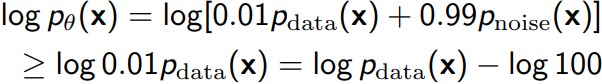
Case 2: Great test log-likelihoods, poor samples. E.g., For a discrete noise mixture model ![]()
- 99% of the samples are just noise
- Taking logs, we get a lower bound
For expected likelihoods, we know that
- Lower bound

- Upper bound (via non-negativity of KL)

As we increase the dimension of x, absolute value of ![]() increases proportionally but log 100 remains constant. Hence,
increases proportionally but log 100 remains constant. Hence, ![]() in very high dimensions
in very high dimensions
https://zhuanlan.zhihu.com/p/27295635
- Given a data distribution
 ,x是一个真实图片,可以Flatten成一个向量,这个向量集合的分布就是。我们需要生成一些也在这个分布内的图片,如果直接就是这个分布的话,怕是做不到的。
 - We have a generated distribution
 parameterized by
  ,这是一个由参数控制的分布,
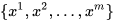
(E.g. is a Gaussian Mixture Model, are means and variances of the Gaussians; - We want to find such that close to
Samples ![]() from
from ![]() ,
,
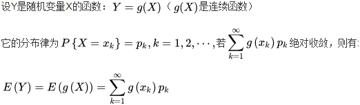
- if given , we can estimate the probability distribution of a future outcome
 :
:  ==> Say you want to estimate the probability that will fall in particular range, You must calculate the integral of the PDF( probability density function, the PDF is a function of x (with θ fixed) ) on this range (i.e., x will fall between –2 and +2, the area of the shaded region,
  )https://blog.csdn.net/Linli522362242/article/details/105973507
 - if given the samples
 , you get Likelihood functions ( ###the likelihood function is a function of θ (with x fixed) ###) of generating the samples:
 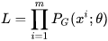 ==>maximize
(i.e. you don’t know θ, observed a single instance x=2.5 (the vertical line, you get the likelihood function ℒ(θ|x=2.5)=f(x=2.5; θ) ==>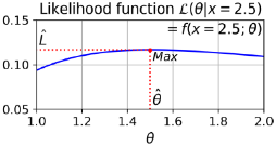 ==> the maximum likelihood estimate (MLE) of θ is
  ; Once you have estimated
  , the value of θ that maximizes the likelihood function, then you are ready to compute
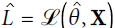
if you observed several independent instances, you would need to find the value of θ that maximizes the product of the individual likelihood functions. But it is equivalent, and much simpler, to maximize the sum (not the product) of the log likelihood functions, thanks to the magic of the logarithm which converts products into sums: log(ab)=log(a)+log(b).)
Here, find ![]() can maximize the likelihood
can maximize the likelihood ![]() and
and ![]()
 因为此时这m个数据
![]() ,是从真实分布
,是从真实分布![]() 中取的,所以也就约等于(approximate)在
中取的,所以也就约等于(approximate)在![]() 分布中得到
分布中得到![]() 的log似然的期望
的log似然的期望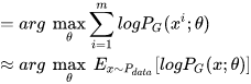 。
。
![]() 分布中得到所有( 也存在于真实分布
分布中得到所有( 也存在于真实分布![]() 的 )X的log似然的期望,等价于求概率积分,所以可以转化成积分运算;此外,因为和减号后面的项无关,所以减掉
的 )X的log似然的期望,等价于求概率积分,所以可以转化成积分运算;此外,因为和减号后面的项无关,所以减掉![]() 中的部分X不在
中的部分X不在![]() 分布中,但在
分布中,但在![]() 分布中的log似然的期望)。
分布中的log似然的期望)。
然后提出共有的项,括号内的反转,max变min,就可以转化为KL divergence的形式了,KL divergence描述的是两个概率分布之间的差异(KL divergence值越小,2个distributions越相近)。https://blog.csdn.net/Linli522362242/article/details/116576478 所以最大化似然,让generator最大概率的生成真实图片,也就是要找一个![]() 让
让![]() 更接近于
更接近于![]() ( We want to find
( We want to find ![]() such that
such that ![]() close to
close to ![]() )
)
How to have very general ![]() ?
?
我们可以假设![]() 是一个神经网络Neural Network。
是一个神经网络Neural Network。
first assume we have a network that receives a random vector, z, sampled from a known distribution(i.e. gaussian distribution or normal distribution) and generates an output image, x. We will call this network generator (G). generator G(z)=x OR G(z; ![]() ) ( generative model 中
) ( generative model 中![]() 值的不同 可以产生各式各样足够复杂的distribution, generated distribution
值的不同 可以产生各式各样足够复杂的distribution, generated distribution ![]() ), 生成图片x,那么我们如何比较两个分布是否相似呢?只要我们取一组sample z,这组z符合一个分布,那么通过网络就可以生成另一个分布
), 生成图片x,那么我们如何比较两个分布是否相似呢?只要我们取一组sample z,这组z符合一个分布,那么通过网络就可以生成另一个分布![]() ,然后来比较与真实分布
,然后来比较与真实分布![]() .
.
 I : identity function, if G(z)=x, and x == x in
 ![]() , the identity function return 1, otherwise, return 0
, the identity function return 1, otherwise, return 0
大家都知道,神经网络只要有非线性激活函数,就可以去拟合任意的函数,那么分布也是一样,所以可以用一直正态分布,或者高斯分布,取样去训练一个神经网络,学习到一个很复杂的分布。
现在我们先固定G,来求解最优的D
 vs
vs 
 ==>
==>
对于一个给定的x,得到最优的D如上图,范围在(0,1)内,把最优的D带入![]() ,可以得到:
,可以得到: ==>
==>
Equation 17-2. KL divergence between the target sparsity p and the actual sparsity q ![]() https://blog.csdn.net/Linli522362242/article/details/116576478
https://blog.csdn.net/Linli522362242/article/details/116576478
==> ==>
==>
JS divergence是KL divergence的对称平滑版本,表示了两个分布之间的差异,这个推导就表明了上面所说的,固定G,![]() 表示两个分布之间的差异,最小值是-2log2,最大值为0。
表示两个分布之间的差异,最小值是-2log2,最大值为0。
现在我们需要找个G,来最小化![]() ,观察上式,当时
,观察上式,当时![]() 能够使得
能够使得![]() 最大值为0 ==>
最大值为0 ==>![]() =log2,G是最优的。
=log2,G是最优的。
接着, D(x) 是有限个(e.g. 给定D1(x), D2(x), D3(x)能够使得![]() 最大, 这个时候
最大, 这个时候![]() 只跟G有关,而G由参数
只跟G有关,而G由参数![]() 控制)
控制) D_i(x) is a the max one (the highest point
![]() )
) minimize
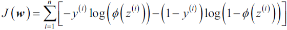
 Minimize 忘记加负号


 ...
...
##########################################https://www.youtube.com/watch?v=0CKeqXl5IY0 OR https://deepgenerativemodels.github.io/notes/gan/
Understanding the loss functions of the generator and discriminator networks in a GAN model
The objective function of GANs, as described in the original paper Generative Adversarial Nets by Goodfellow et al. (https://papers.nips.cc/paper/2014/file/5ca3e9b122f61f8f06494c97b1afccf3-Paper.pdf), is as follows:
The adversarial modeling framework is most straightforward to apply when the models are both multilayer perceptrons. To learn the generator’s distribution ![]() over data x,
over data x,
- we define a prior on input noise variables
 (OR Given a prior distribution ), then represent a mapping to data space as G(z;
  ), where G is a differentiable function represented by a multilayer perceptron with parameters .
 - We also define a second multilayer perceptron D(x;
 ) that outputs a single scalar. D(x) represents the probability that x came from the data rather than
  .
. - We train D to maximize the probability of assigning the correct label to both training examples and samples from the generator (G).
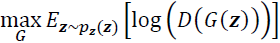
- We simultaneously train G to minimize log(1 − D(G(z))).
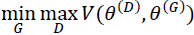
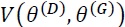
- In other words, D and G play the following two-player minimax game with value function V (G, D):

![]() vs
vs 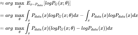
Here, ![]() is called the value function, which can be interpreted as a payoff:
is called the value function, which can be interpreted as a payoff:
- we want to maximize its value with respect to the discriminator (D),
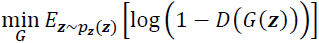
- while minimizing its value with respect to the generator (G), that is,
 . D(x) is the probability that indicates whether the input example, x, is real or fake (that is, generated).(D(x) represents the probability that x came from the real data, 也就是对于x是真实data分布中,D(x)要接近与1,对于x来自于生成的分布,D(x)要接近于0)
The expression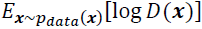 refers to the expected value of the quantity in brackets with respect to the examples from the data distribution (distribution of the real examples);
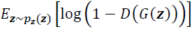 refers to the expected value of the quantity with respect to the distribution of the input, z, vectors (𝒙̃ = 𝐺(𝒛) to refer to the generated output).
One training step of a GAN model with such a value function![]() requires two optimization steps:
requires two optimization steps:
- (1) maximizing the payoff for the discriminator and
- (2) minimizing the payoff for the generator.
A practical way of training GANs is to alternate between these two optimization steps:
- (1) fix (freeze) the parameters of one network and optimize the weights of the other one, and
- (2) fix the second network and optimize the first one.
- This process should be repeated at each training iteration.
Let's assume that the generator network is fixed, and we want to optimize the discriminator.
- Both terms in the value function
 contribute to optimizing the discriminator, where the first term
 corresponds to the loss associated with the real examples, and the second term
 is the loss for the fake examples.
 - Therefore, when G is fixed, our objective is to maximize , which means making the discriminator better at distinguishing between real and generated images.
After optimizing the discriminator using the loss terms for real and fake samples, we then fix the discriminator and optimize the generator.
- In this case, only the second term
 in contributes to the gradients of the generator.
 - As a result, when D is fixed, our objective is to minimize , which can be written as
 <====>
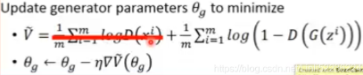
- As was mentioned in the original GAN paper by Goodfellow et al., this function, log(1 − 𝐷(𝐺(𝒛))) , suffers from vanishing gradients消失的梯度 in the early training stages(above right-bottom figure). The reason for this is that the outputs, G(z), early in the learning process, look nothing like real examples, and therefore D(G(z)) will be close to zero with high confidence. This phenomenon is called saturation. To resolve this issue, we can reformulate the minimization objective, , by rewriting it as
 .
.
This replacement![]() means that for training the generator, we can swap the labels of real and fake examples ==> carry out a regular function minimization. In other words, even though the examples synthesized by the generator are fake and are therefore labeled 0, we can flip the labels by assigning label 1 to these examples(fake), and minimize the binary cross-entropy loss with these new labels instead of maximizing
means that for training the generator, we can swap the labels of real and fake examples ==> carry out a regular function minimization. In other words, even though the examples synthesized by the generator are fake and are therefore labeled 0, we can flip the labels by assigning label 1 to these examples(fake), and minimize the binary cross-entropy loss with these new labels instead of maximizing ![]() ==>minimize
==>minimize![]() <==minimize
<==minimize![]() .
.
Now that we have covered the general optimization procedure for training GAN models, let's explore the various data labels that we can use when training GANs. Given that the discriminator is a binary classifier (the class labels are 0 and 1 for fake and real images, respectively), we can use the binary cross-entropy loss function. Therefore, we can determine the ground truth labels for the discriminator loss as follows:![]()
What about the labels to train the generator? As we want the generator to synthesize realistic images, we want to penalize the generator when its outputs are not classified as real by the discriminator. This means that we will assume the ground truth labels for the outputs of the generator to be 1 when computing the loss function for the generator.
Putting all of this together, the following figure displays the individual steps in a simple GAN model:
In the following section, we will implement a GAN from scratch to generate new handwritten digits.
Implementing a GAN from scratch
In this section, we will cover how to implement and train a GAN model to generate new images such as MNIST digits. Since the training on a normal central processing unit (CPU) may take a long time, in the following subsection, we will cover how to set up the Google Colab environment, which will allow us to run the computations on graphics processing units (GPUs).
Training GAN models on Google Colab
Some of the code examples in this chapter may require extensive computational resources that go beyond a commercial laptop or a workstation without a GPU. If you already have an NVIDIA GPU-enabled computing machine available, with CUDA and cuDNN libraries installed, you can use that to speed up the computations.
However, since many of us do not have access to high-performance computing resources, we will use the Google Colaboratory environment (often referred to as Google Colab), which is a free cloud computing service (available in most countries).
Google Colab provides Jupyter Notebook instances that run on the cloud; the notebooks can be saved on Google Drive or GitHub. While the platform provides various different computing resources, such as CPUs, GPUs, and even tensor processing units (TPUs), it is important to highlight that the execution time is currently limited to 12 hours. Therefore, any notebook running longer than 12 hours will be interrupted.
The code blocks in this chapter will need a maximum computing time of two to three hours, so this will not be an issue. However, if you decide to use Google Colab for other projects that take longer than 12 hours, be sure to use checkpointing and save intermediate checkpoints.
Jupyter Notebook
Jupyter Notebook is a graphical user interface (GUI) for running code interactively and interleaving it with text documentation and figures. Due to its versatility[ˌvɜːrsəˈtɪləti]用途广泛 and ease of use, it has become one of the most popular tools in data science.
For more information about the general Jupyter Notebook GUI, please view the official documentation at https://jupyter-notebook.readthedocs.io/en/stable/. All the code in this book is also available in the form of Jupyter notebooks, and a short introduction can be found in the code directory of the first chapter at https://github.com/rasbt/python-machine-learning-book-3rd-edition/tree/master/ch01#pythonjupyter-notebook.
Lastly, we highly recommend Adam Rule et al.'s article Ten simple rules for writing and sharing computational analyses in Jupyter Notebooks on using Jupyter Notebook effectively in scientific research projects, which is freely available at https://journals.plos.org/ploscompbiol/article?id=10.1371/journal.pcbi.1007007.
Accessing Google Colab is very straightforward. You can visit https://colab.research.google.com/, which automatically takes you to a prompt window where you can see your existing Jupyter notebooks. From this prompt window, click the GOOGLE DRIVE tab, as shown in the following figure. This is where you will save the notebook on your Google Drive.
Then, to create a new notebook, click on the link NEW PYTHON 3 NOTEBOOK at the bottom of the prompt window:
This will create and open a new notebook for you. All the code examples you write in this notebook will be automatically saved, and you can later access the notebook from your Google Drive in a directory called Colab Notebooks.
In the next step, we want to utilize GPUs to run the code examples in this notebook. To do this, from the Runtime option in the menu bar of this notebook, click
on Change runtime type and select GPU, as shown in the following figure:
In the last step, we just need to install the Python packages that we will need for this chapter. The Colab Notebooks environment already comes with certain packages, such as NumPy, SciPy, and the latest stable version of TensorFlow. However, at the time of writing, the latest stable version on Google Colab is TensorFlow 1.15.0, but we want to use TensorFlow 2.0. Therefore, first we need to install TensorFlow 2.0 with GPU support by executing the following command in a new cell of this notebook:
! pip install -q tensorflow-gpu==2.0.0(In a Jupyter notebook, a cell starting with an exclamation mark will be interpreted as a Linux shell command.)
Now, we can test the installation and verify that the GPU is available using the following code:
import tensorflow as tf

print( tf.__version__ )![]()
print( "GPU Available:", tf.config.list_physical_devices('GPU') )![]()
if tf.config.list_physical_devices('GPU'):
  device_name = tf.test.gpu_device_name()
else:
  device_name = '/CPU:0'

print(device_name)![]()
Furthermore, if you want to save the model to your personal Google Drive, or transfer or upload other files, you need to mount the Google Drive. To do this, execute the following in a new cell of the notebook:
from google.colab import drive

drive.mount('/content/drive')![]()
This will provide a link to authenticate the Colab Notebook accessing your Google Drive. After following the instructions for authentication, it will provide an authentication code that you need to copy and paste into the designated input field below the cell you have just executed. Then, your Google Drive will be mounted and available at /content/drive/My Drive.
######################################
Leaky rectified linear unit (ReLU) activation function
In Chapter 13, Parallelizing Neural Network Training with TensorFlow, we covered different nonlinear activation functions that can be used in an NN model. If you recall, the ReLU activation function was defined as 𝜙(𝑧) = max(0, 𝑧) , which suppresses the negative (preactivation) inputs; that is, negative inputs are set to zero. As a consequence, using the ReLU activation function may result in sparse gradients during backpropagation. Sparse gradients are not always detrimental and can even benefit models for classification. However, in certain applications, such as GANs, it can be beneficial to obtain the gradients for the full range of input values, which we can achieve by making a slight modification to the ReLU function such that it outputs small values for negative inputs. This modified version of the ReLU function is also known as leaky ReLU. In short, the leaky ReLU activation function permits nonzero gradients for negative inputs as well, and as a result, it makes the networks more expressive overall.
The leaky ReLU activation function is defined as follows: Here, 𝛼 determines the slope for the negative (preactivation) inputs.
######################################
Implementing the generator and the discriminator networks(fully connected layers OR Dense)
We will start the implementation of our first GAN model with a generator and a discriminator as two fully connected networks with one or more hidden layers (see the following figure).
This is the original GAN version, which we will refer to as vanilla GAN.
In this model, for each hidden layer, we will apply the leaky ReLU activation function. The use of ReLU results in sparse gradients(只有少量的神经元被激活: 如果输入值是负的,ReLU函数会转换为0,而神经元不被激活。缺点:x<0时,梯度是零(也存在着梯度为零的问题), 这使得该区域的神经元死亡, 权重无法更新的情况https://blog.csdn.net/Linli522362242/article/details/106935910), which may not be suitable when we want to have the gradients for the full range of input values. In the discriminator network, each hidden layer is also followed by a dropout layer. Furthermore, the output layer in the generator uses the hyperbolic tangent (tanh) activation function. (Using tanh activation is recommended for the generator network since it helps with the learning.)
The output layer in the discriminator has no activation function (that is, linear activation) to get the logits. Alternatively, we can use the sigmoid activation function to get probabilities as output.
We will define two helper functions for each of the two networks, instantiate a model from the Keras Sequential class, and add the layers as described. The code is as
follows:
import tensorflow as tf

## define a function for the generator:
def make_generator_network( num_hidden_layers=1,
                            num_hidden_units=100,
                            num_output_units=784
                          ):
  model = tf.keras.Sequential()
  for i in range( num_hidden_layers ):
    model.add( tf.keras.layers.Dense( units=num_hidden_units,
                                      use_bias=False
                                    )
             ) # fully connected networks
    model.add( tf.keras.layers.LeakyReLU() )

  model.add( tf.keras.layers.Dense( units=num_output_units,
                                    activation="tanh"
                                  )
           )
  return model

## define a function for the discriminator:
def make_discriminator_network( num_hidden_layers=1,
                                num_hidden_units=100,
                                num_output_units=1,
                              ):
  model = tf.keras.Sequential()
  for i in range( num_hidden_layers ):
    model.add( tf.keras.layers.Dense(units=num_hidden_units) )
    model.add( tf.keras.layers.LeakyReLU() )
    model.add( tf.keras.layers.Dropout(rate=0.5) )

  model.add( tf.keras.layers.Dense( units=num_output_units,
                                    activation=None
                                  )
           )
  return model
Next, we will specify the training settings for the model. As you will remember from previous chapters, the image size in the MNIST dataset is 28 × 28 pixels. (That is only one color channel because MNIST contains only grayscale images.) We will further specify the size of the input vector, z, to be 20, and we will use a random uniform distribution to initialize the model weights. Since we are implementing a very simple GAN model for illustration purposes only and using fully connected layers, we will only use a single hidden layer with 100 units in each network. In the following code, we will specify and initialize the two networks, and print their summary information:
import numpy as np

image_size = (28,28)

z_size = 20
model_z = 'uniform' # 'uniform' vs. 'normal

gen_hidden_layers=1
gen_hidden_size=100 # number of hidden units for each hidden layer

disc_hidden_layers=1
disc_hidden_size=100

tf.random.set_seed(1)

gen_model = make_generator_network( num_hidden_layers = gen_hidden_layers,
                                    num_hidden_units = gen_hidden_size,
                                    num_output_units = np.prod(image_size) # 28*28
                                  )
gen_model.build( input_shape=(None, z_size ) )
gen_model.summary()
disc_model = make_discriminator_network( num_hidden_layers=disc_hidden_layers,
                                         num_hidden_units=disc_hidden_size
                                       )
disc_model.build( input_shape=( None, np.prod(image_size) ) )
disc_model.summary()
Defining the training dataset
In the next step, we will load the MNIST dataset and apply the necessary preprocessing steps. Since the output layer of the generator is using the tanh activation function, the pixel values of the synthesized images will be in the range (–1, 1). However, the input pixels of the MNIST images are within the range [0, 255] (with a TensorFlow data type tf.uint8). Thus, in the preprocessing steps, we will use the tf.image.convert_image_dtype function to convert the dtype of the input image tensors from tf.uint8 to tf.float32. As a result, besides changing the dtype, calling this function will also change the range of input pixel intensities to [0, 1](###by / 255.0###). Then, we can scale them by a factor of 2 and shift them by –1 such that the pixel intensities will be rescaled to be in the range [–1, 1]. Furthermore, we will also create a random vector, z, based on the desired random distribution (in this code example, uniform or normal, which are the most common choices), and return both the preprocessed image and the random vector in a tuple:
import tensorflow_datasets as tfds

mnist_bldr = tfds.builder('mnist')
minst_info = mnist_bldr.info
mnist_bldr.download_and_prepare()
mnist = mnist_bldr.as_dataset( shuffle_files=False )
minst_info
import tensorflow_datasets as tfds

mnist_bldr = tfds.builder('mnist')
mnist_bldr.download_and_prepare()
mnist = mnist_bldr.as_dataset( shuffle_files=False )

def preprocess(ex, mode='uniform'):
  image = ex['image']
  image = tf.image.convert_image_dtype( image, tf.float32 ) # /255.0
  image = tf.reshape(image, [-1])
  image = image*2 - 1.0

  if mode == 'uniform':
    input_z = tf.random.uniform( shape=(z_size,),
                                 minval=-1.0,
                                 maxval=1.0
                               )
  elif mode == 'normal':
    input_z = tf.random.normal( shape=(z_size,) ) # mean=0.0, stddev=1.0

  return input_z, image

mnist_trainset = mnist['train']

print("Before preprocessing: ")
example = next( iter(mnist_trainset) )['image']
print('dtype: ', example.dtype, ' Min: {} Max: {}'.format( np.min(example),
                                                           np.max(example)
                                                         )
     )
mnist_trainset = mnist_trainset.map( preprocess )

print('After preprocessing: ')
example = next( iter(mnist_trainset) )[0]
print('dtype: ', example.dtype, ' Min: {} Max: {}'.format( np.min(example),
                                                           np.max(example)
                                                         )
     )
Note that, here, we returned both the input vector, z, and the image to fetch the training data conveniently during model fitting. However, this does not imply that the vector, z, is by any means related to the image—the input image comes from the dataset, while vector z is generated randomly. In each training iteration, the randomly generated vector, z, represents the input that the generator receives for synthesizing a new image, and the images (the real ones as well as the synthesized ones) are the inputs to the discriminator.
Let's inspect the dataset object that we created. In the following code, we will take one batch of examples and print the array shapes of this sample of input vectors and images. Furthermore, in order to understand the overall data flow of our GAN model, in the following code, we will process a forward pass for our generator and discriminator.
First, we will feed the batch of input, z, vectors to the generator and get its output, g_output. This will be a batch of fake examples, which will be fed to the
discriminator model to get the logits for the batch of fake examples, d_logits_fake. Furthermore, the processed images that we get from the dataset object will be fed to the discriminator model, which will result in the logits for the real examples, d_logits_real. The code is as follows:
# mnist_trainset = mnist['train']
# mnist_trainset = mnist_trainset.map( preprocess )
mnist_trainset = mnist_trainset.batch( 32, drop_remainder=True )
input_z, input_real = next( iter(mnist_trainset) )
print( 'input-z -- shape:', input_z.shape )
print( 'input-real -- shape:', input_real.shape )

g_output = gen_model( input_z )
print( 'Output of G -- shape:', g_output.shape )

d_logits_real = disc_model( input_real )
d_logits_fake = disc_model( g_output )
print( 'Disc. (real) -- shape:', d_logits_real.shape )
print( 'Disc. (fake) -- shape:', d_logits_fake.shape )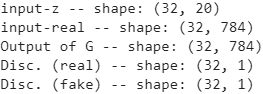
The two logits, d_logits_fake and d_logits_real, will be used to compute the loss functions for training the model(discriminator).
Training the GAN model
As the next step, we will create an instance of BinaryCrossentropy as our loss function and use that to calculate the loss for the generator and discriminator associated with the batches that we just processed. To do this, we also need the ground truth labels for each output.
- For the generator, we will create a vector of 1s with the same shape as the vector containing the predicted logits for the generated images, d_logits_fake.
- For the discriminator loss, we have two terms: the loss for detecting the fake examples involving d_logits_fake and the loss for detecting the real examples based on d_logits_real. The ground truth labels for the fake term will be a vector of 0s that we can generate via the tf.zeros()(or tf.zeros_like()) function. Similarly, we can generate the ground truth values for the real images via the tf.ones()(or tf.ones_like()) function, which creates a vector of 1s:

For the generator : minimize![]()
For the discriminator
Minimize 忘记加负号VS minimize![]() .
.
loss_fn = tf.keras.losses.BinaryCrossentropy( from_logits=True )

## Loss for the Gnerator
# for training the generator, we swap the labels of real and fake examples
# by assigning label 1 to the outputs of the generator
# and minimize the binary cross-entropy loss with these new labels
# when computing the loss function for the generator.
# penalize the generator's outputs those are not classified as real(1)
# by the discriminator(its parameters are fixed (freezed) )
g_labels_real = tf.ones_like( d_logits_fake ) # tf.ones()
g_loss = loss_fn( y_true=g_labels_real,
                  y_pred=d_logits_fake
                )
print( 'Generator Loss: {:.4f}'.format(g_loss) )

## Loss for the Discriminator
d_labels_real = tf.ones_like( d_logits_real ) # tf.ones()
d_labels_fake = tf.zeros_like( d_logits_fake )# tf.zeros()

d_loss_real = loss_fn( y_true=d_labels_real,
                       y_pred=d_logits_real
                     )
d_loss_fake = loss_fn( y_true=d_labels_fake,
                       y_pred=d_logits_fake
                     )
print( 'Discriminator Losses: Real {:.4f} Fake {:.4f}'.format( d_loss_real.numpy(),
                                                               d_loss_fake.numpy()
                                                             )
)![]()
The previous code example shows the step-by-step calculation of the different loss terms for the purpose of understanding the overall concept behind training a GAN model. The following code will set up the GAN model and implement the training loop, where we will include these calculations in a for loop.
In addition, we will use tf.GradientTape() to compute the loss gradients with respect to the model weights and optimize the parameters of the generator and discriminator using two separate Adam optimizers. As you will see in the following code, for alternating between the training of the generator and the discriminator in TensorFlow, we explicitly provide the parameters of each network and apply the gradients of each network separately to the respective designated optimizer:
import time
num_epochs = 100
batch_size = 64
image_size = (28,28)
gen_hidden_layers=1
gen_hidden_size=100
disc_hidden_layers=1
disc_hidden_size=100
tf.random.set_seed(1)
np.random.seed(1)
z_size = 20
mode_z = 'uniform'
######################## 𝒙̂ = 𝑔(𝒛) ########################
if mode_z == 'uniform':
fixed_z = tf.random.uniform( shape=(batch_size, z_size),
minval=-1,
maxval=1
)
elif mode_z == 'normal':
fixed_z = tf.random.normal( shape=(batch_size, z_size) )
######## define a function for the generator ########
# def make_generator_network( num_hidden_layers=1,
# num_hidden_units=100,
# num_output_units=784
# ):
# model = tf.keras.Sequential()
# for i in range( num_hidden_layers ):
# model.add( tf.keras.layers.Dense( units=num_hidden_units, #100
# use_bias=False
# )
# ) # fully connected networks
# model.add( tf.keras.layers.LeakyReLU() )
# model.add( tf.keras.layers.Dense( units=num_output_units, #784
# activation="tanh"
# )
# )
# return model
######## define a function for the discriminator ########
# def make_discriminator_network( num_hidden_layers=1,
# num_hidden_units=100,
# num_output_units=1,
# ):
# model = tf.keras.Sequential()
# for i in range( num_hidden_layers ):
# model.add( tf.keras.layers.Dense(units=num_hidden_units) )#100
# model.add( tf.keras.layers.LeakyReLU() )
# model.add( tf.keras.layers.Dropout(rate=0.5) )
# model.add( tf.keras.layers.Dense( units=num_output_units, #1
# activation=None
# )
# )
# return model
if tf.config.list_physical_devices('GPU'):
device_name = tf.test.gpu_device_name()
else:
device_name = '/CPU:0'
######## set up the model ########
with tf.device( device_name ):
gen_model = make_generator_network( num_hidden_layers=gen_hidden_layers,
num_hidden_units=gen_hidden_size,
num_output_units=np.prod(image_size)
)
gen_model.build( input_shape=(None, z_size) ) # 20
disc_model = make_discriminator_network( num_hidden_layers=disc_hidden_layers,
num_hidden_units=disc_hidden_size
)
disc_model.build( input_shape=( None, np.prod(image_size) ) ) # 784=28*28
def create_samples( g_model, input_z ):
g_output = g_model( input_z, training=False ) # for freezing the generator
images = tf.reshape( g_output, # print( *image_size ) ==> 28 28
(batch_size, *image_size) # (batch_size, image_size) ==> (64, (28, 28))
) # image_size = (28,28) # (batch_size, *image_size) ==> (64, 28, 28)
# since we scaled the pixel intensities by a factor of 2 and shift them by –1
# such that the pixel intensities to be in the range [–1, 1]
return (images+1)/2.0
## Set up the dataset
mnist_trainset = mnist['train']
# def preprocess(ex, mode='uniform'):
# image = ex['image']
# image = tf.image.convert_image_dtype( image, tf.float32 ) # /255.0 and tf.uint8 ==> tf.float32
# image = tf.reshape(image, [-1])
# image = image*2 - 1.0
# if mode == 'uniform':
# input_z = tf.random.uniform( shape=(z_size,),
# minval=-1.0,
# maxval=1.0
# )
# elif mode == 'normal':
# input_z = tf.random.normal( shape=(z_size,) ) # mean=0.0, stddev=1.0
# return input_z, image
mnist_trainset = mnist_trainset.map( lambda ex: preprocess(ex, mode=mode_z) )
# for each instance, return ==> input_z= 𝒙̂ = 𝑔(𝒛), input_real_image_data
mnist_trainset = mnist_trainset.shuffle( 10000 )
mnist_trainset = mnist_trainset.batch( batch_size, drop_remainder=True)
######## Loss function and optimizers ########
loss_fn = tf.keras.losses.BinaryCrossentropy( from_logits=True )
g_optimizer = tf.keras.optimizers.Adam()
d_optimizer = tf.keras.optimizers.Adam()
all_losses = []
all_d_vals = []
epoch_samples=[]
import time
start_time=time.time()
for epoch in range(1, num_epochs+1):
epoch_losses, epoch_d_vals = [],[]
for i, (input_z, input_real) in enumerate( mnist_trainset):
######### Compute generator's Loss ########
with tf.GradientTape() as g_tape:
g_output = gen_model(input_z) #==> 𝒙̂ = 𝑔(𝒛): synthesize realistic images
d_pred_logits_fake = disc_model( g_output, training=False )
# for training the generator, we swap the labels of real and fake examples
# by assigning label 1 to the outputs of the generator
# and minimize the binary cross-entropy loss with these new labels
# when computing the loss function for the generator.
# penalize the generator's outputs those are not classified as real(1)
# by the discriminator(its parameters are fixed (freezed) )
labels_real = tf.ones_like( d_pred_logits_fake )
g_loss = loss_fn( y_true=labels_real,
y_pred= d_pred_logits_fake
)
######## Compute the gradients of g_loss ########
g_grads = g_tape.gradient( g_loss, gen_model.trainable_variables )
g_optimizer.apply_gradients(
grads_and_vars = zip( g_grads, gen_model.trainable_variables)
)
######### Compute discriminator's Loss ########
with tf.GradientTape() as d_tape:
# for real image
d_pred_logits_real = disc_model( input_real, training=True )
d_labels_real = tf.ones_like( d_pred_logits_real )
d_loss_real = loss_fn( y_true=d_labels_real,
y_pred=d_pred_logits_real
)
# for 𝒙̂ = 𝑔(𝒛)
d_pred_logits_fake = disc_model( g_output, training=True )
d_labels_fake = tf.zeros_like( d_pred_logits_fake )
d_loss_fake = loss_fn( y_true=d_labels_fake,
y_pred=d_pred_logits_fake
)
d_loss = d_loss_real + d_loss_fake
######## Compute the gradients of d_loss ########
d_grads = d_tape.gradient( d_loss, disc_model.trainable_variables )
d_optimizer.apply_gradients(grads_and_vars=zip(d_grads,
disc_model.trainable_variables
)
)
epoch_losses.append( ( g_loss.numpy(),
d_loss.numpy(),
d_loss_real.numpy(),
d_loss_fake.numpy()
)# for each batch
)
d_probs_real = tf.reduce_mean( tf.sigmoid( d_pred_logits_real ) ) # for each batch
d_probs_fake = tf.reduce_mean( tf.sigmoid( d_pred_logits_fake ) )
epoch_d_vals.append( ( d_probs_real.numpy(),
d_probs_fake.numpy()
) # for each batch
)
all_losses.append( epoch_losses ) # for each epoch
all_d_vals.append( epoch_d_vals )
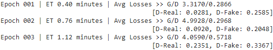
print( 'Epoch {:03d} | ET {:.2f} minutes | Avg Losses >> G/D {:.4f}/{:.4f}'\
'\n\t\t\t\t\t[D-Real: {:.4f}, D-Fake: {:.4f}]'.format(
epoch,
( time.time()-start_time )/60,
*list( np.mean( all_losses[-1], # the latest epoch
axis=0
) # mean of all batches the latest epoch
)
)
)
epoch_samples.append( create_samples( gen_model, fixed_z ).numpy() )
# next epochNote that the discriminator model outputs logits, but for later visualization, we already stored the probabilities computed via the sigmoid function before calculating the averages for each batch.
After each epoch, we generated some examples by calling the create_samples() function and stored them in a Python list
... ...
import pickle
pickle.dump({ 'all_losses': all_losses,
              'all_d_vals': all_d_vals,
              'samples': epoch_samples
            },
            open('/content/drive/My Drive/Colab Notebooks/checkpoints/cp17-vanila-learning.pkl','wb')
            )
gen_model.save('/content/drive/My Drive/Colab Notebooks/models/cp17-vanila-gan_generator.h5')
disc_model.save('/content/drive/My Drive/Colab Notebooks/models/cp17-vanila-gan_discriminator.h5')
Using a GPU, the training process that we implemented in the previous code block should be completed in less than an hour on Google Colab. (It may even be faster on your personal computer if you have a recent and capable CPU and a GPU.) After the model training has completed, it is often helpful to plot the discriminator and generator losses to analyze the behavior of both subnetworks and assess whether they converged.
It is also helpful to plot the average probabilities of the batches of real and fake examples as computed by the discriminator in each iteration. We expect these probabilities to be around 0.5, which means that the discriminator is not able to confidently distinguish between real and fake images:
import itertools
import matplotlib.pyplot as plt
%matplotlib inline

fig = plt.figure( figsize=(16,6) )

## Plotting the losses
ax = fig.add_subplot(1,2,1)
# chain('ABC', 'DEF') --> A B C D E F
# *(( g_loss, d_loss, d_loss_real, d_loss_fake ),...)==>
# ( g_loss, d_loss, d_loss_real, d_loss_fake ), ...
# chain ==> iter( g_loss, d_loss, d_loss_real, d_loss_fake )
g_losses = [ item[0] for item in itertools.chain(*all_losses) ]
d_losses = [ item[1]/2.0 for item in itertools.chain(*all_losses) ] # (d_loss_real + d_loss_fake)/2.0
plt.plot( g_losses, label='Generator Loss', alpha=0.95 )
plt.plot( d_losses, label="Discriminator Loss", alpha=0.95 )
plt.legend( fontsize=20 )
ax.set_xlabel('Iteration', size=15)
ax.set_ylabel("Loss", size=15)

# epochs=np.arange(1, 101)

epoch2iter = lambda e: e*len(all_losses[-1]) # all_losses[-1] : last epoch
epoch_ticks = [1,20,40,60,80,100]
newpos = [epoch2iter(e) for e in epoch_ticks]

ax2=ax.twiny()
ax2.set_xticks( newpos )
ax2.set_xticklabels( epoch_ticks ) # [1,20,40,60,80,100]
ax2.xaxis.set_ticks_position('bottom')
ax2.xaxis.set_label_position('bottom')
# ax.spines[‘bottom’]获取底部的轴,通过set_position方法,设置底部轴的位置,
# outward:向绘图窗外
ax2.spines['bottom'].set_position(('outward', 60))
ax2.set_xlabel("Epoch", size=15)
ax2.set_xlim( ax.get_xlim() )
ax.tick_params( axis='both', which='major', labelsize=15 )
ax2.tick_params( axis='both', which='major', labelsize=15 )

##Plotting the outputs of the discriminator
ax = fig.add_subplot(1,2,2)
d_vals_real = [ item[0] for item in itertools.chain(*all_d_vals) ]
d_vals_fake = [ item[1] for item in itertools.chain(*all_d_vals) ]
plt.plot( d_vals_real, alpha=0.75, label=r'Real: $D(\mathbf{x})$' ) # b: bold
plt.plot( d_vals_fake, alpha=0.75, label=r'Fake: $D(G(\mathbf{z}))$' )
plt.legend(fontsize=20)
ax.set_xlabel('Iteration', size=15)
ax.set_ylabel('Discriminator output', size=15)

ax2=ax.twiny()
ax2.set_xticks(newpos)
ax2.set_xticklabels(epoch_ticks) # [1,20,40,60,80,100]
ax2.xaxis.set_ticks_position('bottom')
ax2.xaxis.set_label_position('bottom')
ax2.spines['bottom'].set_position(('outward', 60))
ax2.set_xlabel('Epoch', size=15)
ax2.set_xlim( ax.get_xlim() ) ######
ax.tick_params(axis='both', which='major', labelsize=15)
ax2.tick_params(axis='both', which='major', labelsize=15)
The following figure shows the results:
 vs
vs 
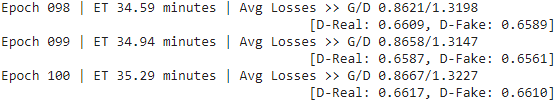
As you can see from the discriminator outputs in the previous figure,
- during the early stages of the training, the discriminator was able to quickly learn to distinguish quite accurately between the real and fake examples, that is, the fake examples had probabilities close to 0, and the real examples had probabilities close to 1. The reason for that was that the fake examples were nothing like the real ones; therefore, distinguishing between real and fake was rather easy.
- As the training proceeds further, the generator will become better at synthesizing realistic images, which will result in probabilities of both real and fake examples that are close to 0.5.
Furthermore, we can also see how the outputs of the generator, that is, the synthesized images, change during training. After each epoch, we generated some examples by calling the create_samples() function and stored them in a Python list. In the following code, we will visualize some of the images produced by the generator for a selection of epochs:
selected_epochs = [1,2,4,10,50,100]
fig = plt.figure( figsize=(10,14) )
for i,e in enumerate( selected_epochs ):
  for j in range(5):
    ax = fig.add_subplot( 6,5, i*5 + j+1)
    ax.set_xticks([])
    ax.set_yticks([])
    if j==0:
      ax.text( -0.06, 0.5, #the anchor point of textbox(move to left by 0.06, move to up by 0.5)
               'Epoch {}'.format(e), rotation=90, size=18, color='red',
               horizontalalignment='right',#the anchor point horizontal axis
               verticalalignment='center', #the anchor point vertical axis
               transform=ax.transAxes )# move the anchor point to (-0.06, 0.5)
    image = epoch_samples[e-1][j]
    ax.imshow(image, cmap='gray_r')

plt.show()
The following figure shows the produced images:
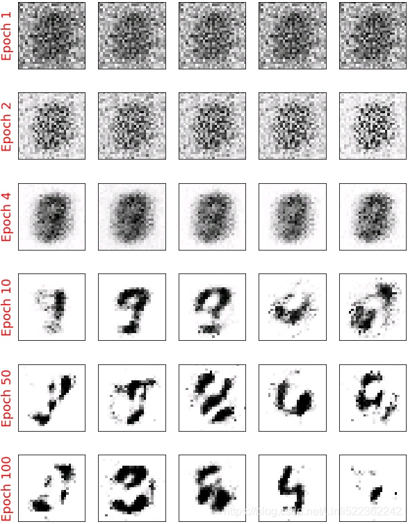
As you can see from the previous figure, the generator network produced more and more realistic images as the training progressed. However, even after 100 epochs, the produced images still look very different to the handwritten digits contained in the MNIST dataset.
In this section, we designed a very simple GAN model with only a single fully connected hidden layer for both the generator and discriminator. After training the GAN model on the MNIST dataset, we were able to achieve promising, although not yet satisfactory, results with the new handwritten digits. As we learned in Chapter
15, Classifying Images with Deep Convolutional Neural Networks, NN architectures with convolutional layers have several advantages over fully connected layers when it comes to image classification. In a similar sense, adding convolutional layers to our GAN model to work with image data might improve the outcome. In the next section, we will implement a deep convolutional GAN (DCGAN), which uses convolutional layers for both the generator and the discriminator networks.
Improving the quality of synthesized images using a convolutional and Wasserstein GAN
https://blog.csdn.net/Linli522362242/article/details/117370337


 2636
2636


 被折叠的 条评论
为什么被折叠?
被折叠的 条评论
为什么被折叠?
 到【灌水乐园】发言


