cp17_2GAN for Synthesizing_upsample_Transposed_Batch normalization_DCGAN_KL_JS divergence_双轴_EM_tape

cp17_GAN for Synthesizing Data_fully connected layer 2 convolutional_colab_ax.transAxes_twiny_spine: https://blog.csdn.net/Linli522362242/article/details/116565829

Improving the quality of synthesized images using a convolutional and Wasserstein GAN

     In this section, we will implement a DCGAN, which will enable us to improve the performance we saw in the previous GAN example. Additionally, we will employ several extra key techniques and implement a Wasserstein GAN (WGAN).

The techniques that we will cover in this section will include the following:

• • Transposed convolution
• • BatchNorm
• • WGAN
• • Gradient penalty

     The DCGAN was proposed in 2016 by A. Radford, L. Metz, and S. Chintala in their article Unsupervised representation learning with deep convolutional generative adversarial
networks, which is freely available at https://arxiv.org/pdf/1511.06434.pdf. In this article, the researchers proposed using convolutional layers for both the generator and discriminator networks. Starting from a random vector, z, the DCGAN first uses a fully connected layer to project z into a new vector with a proper size so that it can be reshaped into a spatial convolution representation (ℎ × 𝑤 × 𝑐 ), which is smaller than the output image size. Then, a series of convolutional layers, known as transposed convolution, are used to upsample the feature maps to the desired output image size.

Transposed convolution

     In Chapter 15, Classifying Images with Deep Convolutional Neural Networks, you learned about the convolution operation in one- and two-dimensional spaces. In particular, we looked at how the choices for the padding and strides change the output feature maps. While a convolution operation is usually used to downsample the feature space (for example, by setting the stride to 2, or by adding a pooling layer after a convolutional layer), a transposed convolution operation is usually used for upsampling the feature space.

     To understand the transposed convolution operation, let's go through a simple thought experiment. Assume that we have an input feature map of size 𝑛 × 𝑛 . Then, we apply a 2D convolution operation with certain padding and stride parameters to this 𝑛 × 𝑛 input, resulting in an output feature map of size 𝑚 × 𝑚 . Now, the question is, how we can apply another convolution operation to obtain a feature map with the initial dimension 𝑛 × 𝑛 from this 𝑚 × 𝑚 output feature map while maintaining the connectivity patterns between the input and output? Note that only the shape of the 𝑛 × 𝑛 input matrix is recovered and not the actual matrix values. This is what transposed convolution does, as shown in the following figure: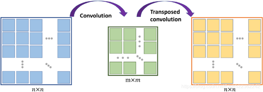

###########################################

Transposed convolution versus deconvolution

     Transposed convolution is also called fractionally strided convolution. In deep learning literature, another common term that is used to refer to transposed convolution is deconvolution. However, note that deconvolution was originally defined as the inverse of a convolution operation, f, on a feature map, x, with weight parameters, w, producing feature map 𝒙′, . A deconvolution function, , can then be defined as . However, note that the transposed convolution is merely focused on recovering the dimensionality of the feature space and not the actual values.
###########################################

     Upsampling feature maps using transposed convolution works by inserting 0s between the elements of the input feature maps. The following illustration shows an example of

• applying transposed convolution to an input of size 4 × 4 , with a stride of 2 × 2 and kernel size of 2 × 2 .

  # Upscaled Image
  stride = 2, kernel size=2
  (height-1)*stride + 2*kernel_size-1, # e.g. (4-1)*2 + 2*2 -1 = 9
  (width-1) *stride + 2*kernel_size-1, # e.g. (4-1)*2 + 2*2 -1 = 9

  # code
    upscaled = np.zeros( ( batch_size,
                           (height-1)*stride + 2*kernel_size-1, # e.g. (4-1)*2 + 2*2 -1 = 9
                           (width-1) *stride + 2*kernel_size-1, # e.g. (4-1)*2 + 2*2 -1 = 9
                           channels
                         ) )

  # then assign the original image values to the upscaled image
    upscaled[:, # batch_size
                   kernel_size-1:(height-1)*stride + kernel_size:stride, # 2-1:(4-1)*2+2:2 ==> 1:8:2
                   kernel_size-1:(width-1) *stride + kernel_size:stride, # 2-1:(4-1)*2+2:2 ==> 1:8:2
                  :]=images

• The matrix of size 9 × 9 in the center shows the results after inserting such 0s into the input feature map.
• Then, performing a normal convolution using the 2 × 2 kernel with a new stride of 1 results in an output of size 8 × 8 .
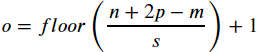  padding="VALID" since 9 × 9 != 8 × 8 ==> padding=0
• We can verify the backward direction by performing a regular convolution on the output with a stride of 2, which results in an output feature map of size 4 × 4 (8/2=4), which is the same as the original input size:

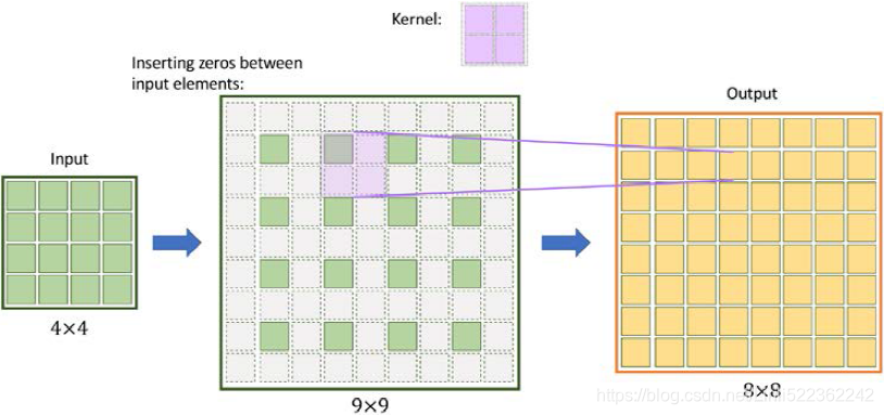
Another example:

https://blog.csdn.net/Linli522362242/article/details/108669444

• applying transposed convolution to an input of size 2 × 3 , with a stride of 2 × 2 and kernel size of 3 × 3 .

  # Upscaled Image
  stride = 2, kernel size=3
  (height-1)*stride + 2*kernel_size-1, # e.g. (3-1)*2 + 2*3 -1 = 9
  (width-1) *stride + 2*kernel_size-1, # e.g. (2-1)*2 + 2*3 -1 = 7

  # code
    upscaled = np.zeros( ( batch_size,
                           (height-1)*stride + 2*kernel_size-1, # e.g. (3-1)*2 + 2*3 -1 = 9
                           (width-1) *stride + 2*kernel_size-1, # e.g. (2-1)*2 + 2*3 -1 = 7
                           channels
                         ) )

  # then assign the original image values to the upscaled image  upscaled[:, # batches
                   kernel_size-1:(height-1)*stride + kernel_size:stride, # 3-1:(3-1)*2+3:2 ==> 2:7:2
                   kernel_size-1:(width-1) *stride + kernel_size:stride, # 3-1:(2-1)*2+3:2 ==> 2:5:2
                  :]=images

• The matrix of size 7 × 9 in the center shows the results after inserting such 0s into the input feature map
• Then, performing a normal convolution using the 3 × 3 kernel with a new stride of 1 results in an output of size 5 × 7 .
  padding="VALID" since 7 × 9 != 5 × 7  ==>p=1
• We can verify the backward direction by performing a regular convolution on the output with a stride of 2, which results in an output feature map of size 2 × 3 (5/2=2, 7/2=3), which is the same as the original input size:

     The preceding illustration shows how transposed convolution works in general. There are various cases in which input size, kernel size, strides, and padding variations can change the output. If you want to learn more about all these different cases, refer to the tutorial A Guide to Convolution Arithmetic for Deep Learning by Vincent Dumoulin and Francesco Visin, which is freely available at https://arxiv.org/pdf/1603.07285.pdf.

Batch normalization

     BatchNorm was introduced in 2015 by Sergey Ioffe and Christian Szegedy in the article Batch Normalization: Accelerating Deep Network Training by Reducing Internal Covariate Shift, which you can access via arXiv at https://arxiv.org/pdf/1502.03167.pdf. One of the main ideas behind BatchNorm is normalizing the layer inputs and preventing changes in their distribution during training, which enables faster and better convergence.

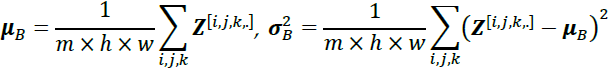
     BatchNorm transforms a mini-batch of features based on its computed statistics. Assume that we have the net preactivation feature maps obtained after a convolutional layer in a four-dimensional tensor, Z, with the shape [𝑚 × ℎ × 𝑤 × 𝑐], where m is the number of examples in the batch (i.e., batch size), ℎ × 𝑤 is the spatial dimension of the feature maps, and c is the number of channels. BatchNorm can be summarized in three steps, as follows:

• 1. Compute the mean and standard deviation of the net inputs for each minibatch:
  ),
  where and  both have size c. and c is the number of channels
   is the vector of input means, evaluated over the whole mini-batch B (it contains one mean per input).
   is the vector of input standard deviations, also evaluated over the whole minibatch B(it contains one standard deviation per input).
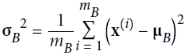
  输入m个样本，每个样本的通道数为c，空间维度为h*w， 先在空间维度（所有特征维度）做归一化期间得到，然后再对所有样本做归一化，期间得到和；或者先对𝑚 × ℎ × 𝑤求和，然后求平均和标准差，最后下一个通道。
• 2. Standardize the net inputs for all examples in the batch: 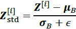 ,where 𝜖 is a small number for numerical stability (that is, to avoid division by zero, (typically ). This is called a smoothing term.
   is the vector of zero-centered( and unit variance) and normalized inputs for instance i.
• 3. Scale and shift the normalized net inputs using two learnable parameter vectors, 𝜸 and 𝜷 , of size c (number of channels): .
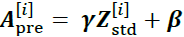  𝜸 is the output scale parameter vector for the layer (it contains one scale parameter per input feature).
  𝜷 is the output shift (offset) parameter vector for the layer (it contains one offset parameter per input). Each input is offset by its corresponding shift parameter.
  𝜸 (the output scale vector) and 𝜷 (the output offset vector) are learned through regular backpropagation

The following figure illustrates the process: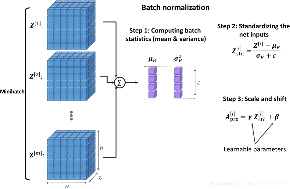
In the first step of BatchNorm, the mean, , and standard deviation, , of the minibatch are computed. Both and are vectors of size c (where c is the number of channels). Then, these statistics are used in step 2 to scale the examples in each mini-batch via z-score normalization (standardization), resulting in standardized net inputs, . As a consequence,

• these net inputs are mean-centered and have unit variance, which is generally a useful property for gradient descent-based optimization.
• On the other hand, always normalizing the net inputs such that they have the same properties across the different mini-batches, which can be diverse, can severely impact the representational capacity of NNs. This can be understood by considering a feature, 𝑥 ∼ 𝑁(0,1) , which, after sigmoid activation to 𝜎(𝑥) , results in a linear region for values close to 0.

Therefore, in step 3, the learnable parameters, 𝜷 and 𝜸 , which are vectors of size c (number of channels), allow BatchNorm to control the shift and spread of the normalized features.https://blog.csdn.net/Linli522362242/article/details/106935910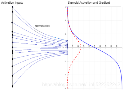

During training, the running averages, , and running variance, , are computed, which are used along with the tuned parameters, 𝜷 and 𝜸 , to normalize the test
example(s) at evaluation. OR https://blog.csdn.net/Linli522362242/article/details/106935910 most implementations of Batch Normalization estimate these final statistics during training by using a moving average of the layer’s input means and standard deviations. This is what Keras does automatically when you use the BatchNormalization layer.  To sum up, four parameter vectors are learned in each batch-normalized layer: γ (the output scale vector) and β (the output offset vector) are learned through regular backpropagation https://blog.csdn.net/Linli522362242/article/details/111940633, and μ (the final input mean vector) and σ (the final input standard deviation vector) are estimated using an exponential moving average. Note that μ and σ are estimated during training, but they are used only after training (to replace the batch input means and standard deviations.

################################

Why does BatchNorm help optimization?

     Initially, BatchNorm was developed to reduce the so-called internal covariance shift, which is defined as the changes that occur in the distribution of a layer's activations due to the updated network parameters during training.

     To explain this with a simple example, consider a fixed batch that passes through the network at epoch 1. We record the activations of each layer for this batch. After iterating through the whole training dataset and updating the model parameters, we start the second epoch, where the previously fixed batch passes through the network. Then, we compare the layer activations from the first and second epochs. Since the network parameters have changed, we observe that the activations have also changed. This phenomenon is called the internal covariance shift, which was believed to decelerate减速 NN training.

     However, in 2018, S. Santurkar, D. Tsipras, A. Ilyas, and A. Madry further investigated what makes BatchNorm so effective. In their study, the researchers observed that the effect of BatchNorm on the internal covariance shift is marginal. Based on the outcome of their experiments, they hypothesized that the effectiveness of BatchNorm is, instead, based on a smoother surface of the loss function, which makes the non-convex optimization more robust.

     If you are interested in learning more about these results, read through the original paper, How Does Batch Normalization Help Optimization?, which is freely available at http://papers.nips.cc/paper/7515-how-does-batch-normalizationhelp-optimization.pdf. OR  https://proceedings.neurips.cc/paper/2018/file/905056c1ac1dad141560467e0a99e1cf-Paper.pdf.
################################

     The TensorFlow Keras API provides a class, tf.keras.layers. BatchNormalization(), that we can use as a layer when defining our models; it will perform all of the steps that we described for BatchNorm. Note that the behavior for updating the learnable parameters, 𝜸 and 𝜷 , depends on whether training=False or training=True, which can be used to ensure that these parameters are learned only during training.

Implementing the generator and discriminator

################################

Architecture design considerations for convolutional GANs

     Notice that the number of feature maps follows different trends between the generator and the discriminator. In the generator, we start with a large number of feature maps and decrease them as we progress toward the last layer. On the other hand, in the discriminator, we start with a small number of channels and increase it toward the last layer. This is an important point for designing CNNs with the number of feature maps and the spatial size of the feature maps in reverse order. When the spatial size of the feature maps increases, the number of feature maps decreases and vice versa.

     In addition, note that it's usually not recommended to use bias units in the layer that follows a BatchNorm layer. Using bias units would be redundant in this case, since BatchNorm already has a shift parameter, 𝜷 . You can omit the bias units for a given layer by setting use_bias=False in tf.keras.layers.Dense or tf.keras.layers.Conv2D.

################################

import tensorflow as tf
import tensorflow_datasets as tfds
import numpy as np
import matplotlib.pyplot as plt
%matplotlib inline

print(tf.__version__)
print( "GPU Available:", tf.config.list_physical_devices('GPU') )

if tf.config.list_physical_devices('GPU'):
  device_name = tf.test.gpu_device_name()
else:
  device_name = 'CPU:0'

print( device_name )

     At this point, we have covered the main components of a DCGAN model, which we will now implement. The architectures of the generator and discriminator networks are summarized in the following two figures.

The generator

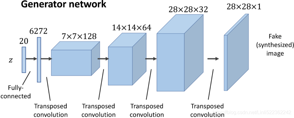
• takes a vector, z, of size 20 as input,
• applies a fully connected (dense) layer to increase its size to 6,272 and
• then reshapes it into a rank-3 tensor of shape 7 × 7 × 128 (spatial dimension 7 × 7 and 128 channels).
• Then, a series of transposed convolutions using tf.keras.layers.Conv2DTransposed() upsamples the feature maps until the spatial dimension of the resulting feature maps reaches 28 × 28 .
  The number of channels is reduced by half after each transposed convolutional layer, except the last one, which uses only one output filter to generate a grayscale image.
  Each transposed convolutional layer is followed by BatchNorm and leaky ReLU activation functions, except the last one, which uses tanh activation (without BatchNorm).
• The architecture for the generator (the feature maps after each layer) is shown in the previous figure.

def make_dcgan_generator( z_size=20,
                          output_size=(28,28,1),
                          n_filters=128,
                          n_blocks=2
                        ):
  size_factor = 2**n_blocks                    # 2**2=4
  hidden_size = ( output_size[0]//size_factor, # 28//4=7
                  output_size[1]//size_factor  # 28//4=7 
                )
  model = tf.keras.Sequential([ 
                    tf.keras.layers.InputLayer( input_shape=(z_size,) ), # 128*7*7=6272
                    tf.keras.layers.Dense( units=n_filters*np.prod(hidden_size),
                                           use_bias=False # bias is redundant since the follow BatchNorm in which already has a shift parameter, 𝜷
                                         ), # Fully connected
                    tf.keras.layers.BatchNormalization(),
                    tf.keras.layers.LeakyReLU(),
                    tf.keras.layers.Reshape(
                        (hidden_size[0], hidden_size[1], n_filters) # 7,7,128
                    ),
                    tf.keras.layers.Conv2DTranspose(
                        filters=n_filters,             # 128
                        kernel_size=(5,5), 
                        strides=(1,1), padding='same', # ==> output shape: (7,7,128) 
                        use_bias=False
                    ),
                    tf.keras.layers.BatchNormalization(),
                    tf.keras.layers.LeakyReLU()           
          ])
  # When the spatial size of the feature maps increases, the number of feature maps decreases and vice versa
  nf = n_filters
  for i in range( n_blocks ):
    nf = nf//2                                 # 128//2=64
    model.add( tf.keras.layers.Conv2DTranspose( 
                                filters=nf,    # 64 ==>32
                                kernel_size=(5,5), 
                                strides=(2,2), padding='same', # ==> output shape: (14,14,filters=64) ==> (28,28,filters=32)
                                use_bias=False)
             )
    model.add( tf.keras.layers.BatchNormalization() )
    model.add( tf.keras.layers.LeakyReLU() )
  
  model.add(
      tf.keras.layers.Conv2DTranspose(
          filters=output_size[2],        # 1
          kernel_size=(5,5),
          strides=(1,1), padding='same', # ==> output shape: (28,28,filters=1)
          use_bias=False,
          activation='tanh' # tanh activation is recommended for the generator network since it helps with the learning
      )
  )
  return model

We can create the generator networks using the helper function, make_dcgan_generator(), and print its architecture as follows: 

gen_model = make_dcgan_generator()
gen_model.summary()

 

The discriminator

 

• receives images of size 28 × 28 × 1 , which are passed through 4 convolutional layers.
• The first three convolutional layers reduce the spatial dimensionality by 4 while increasing the number of channels of the feature maps.
  Each convolutional layer is also followed by BatchNorm, leaky ReLU activation, and a dropout layer with rate=0.3 (drop probability).
  The last convolutional layer uses kernels of size 7 × 7 and a single filter to reduce the spatial dimensionality of the output to 1 × 1 × 1.

def make_dcgan_discriminator( input_size=(28,28,1),
                              n_filters=64,
                              n_blocks=2
                            ):
  model = tf.keras.Sequential([
                    tf.keras.layers.InputLayer( input_shape=input_size ),
                    tf.keras.layers.Conv2D( filters=n_filters,
                                            kernel_size=5,
                                            strides=1,
                                            padding='same', # output shape: (28,28,filters=64)
                                            use_bias=True
                                          ),
                    tf.keras.layers.BatchNormalization(),
                    tf.keras.layers.LeakyReLU()                      
          ])
  nf = n_filters
  for i in range(n_blocks):
    nf = nf*2
    model.add( tf.keras.layers.Conv2D( filters=nf, # 128 ==> 256
                                       kernel_size=(5,5), 
                                       strides=(2,2), padding='same', # ==> output shape: (14,14,filters=128) ==> (7,7,filters=256)
                                       use_bias=True
                                     )
             )
    model.add( tf.keras.layers.BatchNormalization() )
    model.add( tf.keras.layers.LeakyReLU() )
    model.add( tf.keras.layers.Dropout(0.3) )
  
  model.add( tf.keras.layers.Conv2D( filters=1, 
                                     kernel_size=(7,7), strides=(1,1), # output shape:  (1,1,filters=1)
                                     padding='valid', 
                                     use_bias=True
                                   )
           )
  model.add( tf.keras.layers.Reshape( (1,) ) ) # class probability

  return model

Similarly, we can generate the discriminator network and see its architecture: 

disc_model = make_dcgan_discriminator()
disc_model.summary()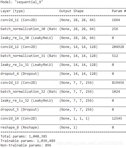

 Notice that the number of parameters for the BatchNorm layers is indeed 4 times the number of channels (4 × channels ).  e.g. 256=4*64, 512= 4*128, 1024=4*256. Remember that the BatchNorm parameters,

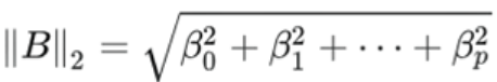
• and , represent the (non-trainable parameters, 896=(256+512+1024)/2 = 1792/2) mean and standard deviation for each feature value inferred from a given batch;
• 𝜸 and 𝜷 are the trainable BN parameters.

     With these two helper functions(make_dcgan_generator and make_dcgan_discriminator), you can build a DCGAN model and train it by using the same MNIST dataset object we initialized in the previous section when we implemented the simple, fully connected GAN https://blog.csdn.net/Linli522362242/article/details/116565829. Also, we can use the same loss functions and training procedure as before.

     Note that this particular architecture would not perform very well when using cross-entropy as a loss function.

     In the next subsection, we will cover WGAN, which uses a modified loss function based on the so-called Wasserstein-1 (or earth mover's) distance between the distributions of real and fake images for improving the training performance.

#############################

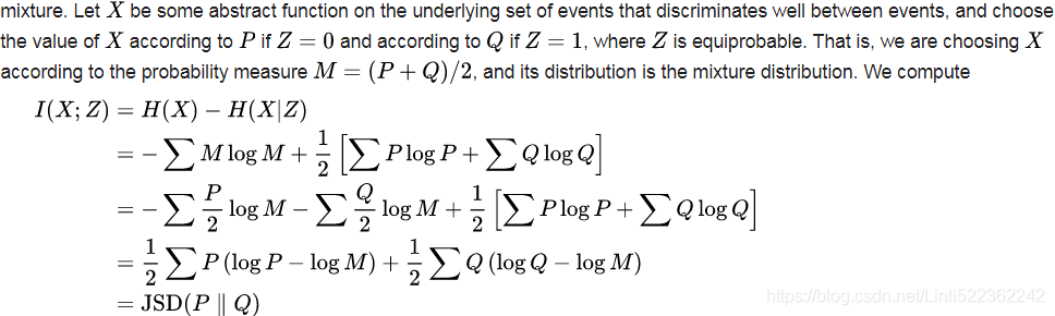
The relationship between KL divergence and cross-entropy

     KL divergence, 𝐾L(𝑃‖𝑄) , measures the relative entropy of the distribution, P, with respect to a reference distribution, Q. The formulation for KL divergence can be extended as 

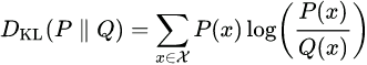Moreover, for discrete probability distributions( P and Q defined on the same probability space, , the relative entropy from Q to P is defined to be,  or(KL divergence)
which can be similarly extended as or 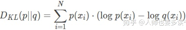 也就是说，q(x)能在多大程度上表达p(x)所包含的信息，KL散度越大，表达效果越差https://blog.csdn.net/Linli522362242/article/details/116576478

可将该式写作期望的形式 
     Based on the extended formulation (either discrete or continuous), KL divergence is viewed as the cross-entropy between P and Q (the first term in the preceding equation) subtracted by the (self-) entropy of P (second term), that is, 𝐾L(𝑃‖𝑄) = 𝐻(𝑃, 𝑄) − 𝐻(𝑃) .
#############################

Dissimilarity measures between two distributions

     We will first see different measures for computing the divergence between two distributions. Then, we will see which one of these measures is already embedded in the original GAN model. Finally, switching this measure in GANs will lead us to the implementation of a WGAN.

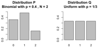
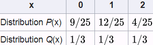
     As mentioned at the beginning of this chapter, the goal of a generative model is to learn how to synthesize new samples that have the same distribution as the distribution of the training dataset. Let P(x) and Q(x) represent the distribution of a random variable, x, as shown in the following figure.

     First, let's look at some ways, shown in the following figure, that we can use to measure the dissimilarity between two distributions, P and Q: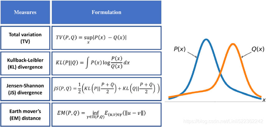

     The function supremum, sup(S), used in the total variation (TV) measure, refers to the smallest value that is greater than all elements of S. In other words, sup(S) is the least upper bound for S. Vice versa, the infimum function, inf(S), which is used in EM distance, refers to the largest value that is smaller than all elements of S (the greatest lower bound). Let's gain an understanding of these measures by briefly stating what they are trying to accomplish in simple words:

• • The first one, TV distance, measures the largest difference between the two distributions at each point.
  
   : ,
• • The EM distance can be interpreted as the minimal amount of work needed to transform one distribution into the other.
       The infimum function极小函数 in the EM distance is taken over (P, Q) , which is the collection of all joint distributions 𝛾(𝑢, 𝑣) whose marginals are P or Q.
       Then, 𝛾(𝑢, 𝑣) is a transfer plan, which indicates how we redistribute the earth from location u to v (Intuitively,  𝛾(𝑢, 𝑣) indicates how much “mass” must be transported from 𝑢 to 𝑣 in order to transform the distributions P into the distribution Q), subject to some constraints for maintaining valid distributions after such transfers.
       Computing EM distance is an optimization problem by itself, which is to find the optimal transfer plan, 𝛾(𝑢, 𝑣) .OR The EM distance then is the “cost” of the optimal transport plan.
  
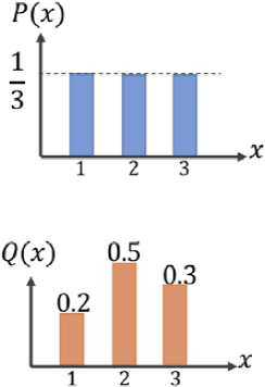
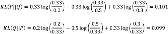
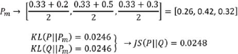
       Note that, in the case of the EM distance, for this simple example, we can see that Q(x) at x = 2 has the excess value of 0.5− 1/3= 0.166 , while the value of Q at the other two x's is below 1/3. Therefore, the minimal amount of work is when we transfer the extra value at x = 2 to x = 1 and x = 3
• • The Kullback-Leibler (KL) and Jensen-Shannon (JS) divergence分歧 measures come from the field of information theory. Note that KL divergence is not symmetric, that is, 𝐾L(𝑃‖𝑄) ≠ 𝐾L(𝑄‖𝑃) in contrast to JS divergence.

<==

Relative entropies  and  are calculated as follows. This example uses the natural log with base e, designated ln to get results in nats (see units of information).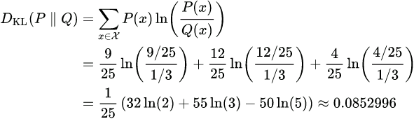
Q(x)能在多大程度上 表达P(x)所包含的信息(这儿是)，KL散度越大，表达效果越差
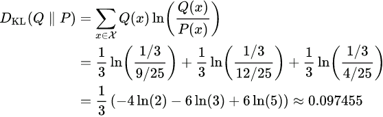
Note that KL divergence is not symmetric, that is, 𝐾L(𝑃‖𝑄) ≠ 𝐾L(𝑄‖𝑃) in contrast to JS divergence.

• Jensen-Shannon (JS) divergence Is a symmetrized and smoothed version of the Kullback–Leibler divergence . It is defined by  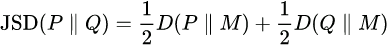where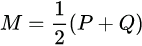 
  

==>https://en.wikipedia.org/wiki/Jensen%E2%80%93Shannon_divergence

The dissimilarity equations provided in the previous figure correspond to continuous distributions but can be extended for discrete cases. An example of calculating these different dissimilarity measures with two simple discrete distributions is illustrated in the following figure: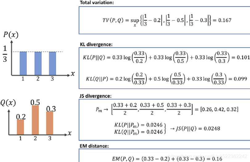
 Note that, in the case of the EM distance, for this simple example, we can see that Q(x) at x = 2 has the excess value of 0.5− 1/3= 0.166 , while the value of Q at the other two x's is below 1/3. Therefore, the minimal amount of work is when we transfer the extra value at x = 2 to x = 1 and x = 3, as shown in the previous figure. For this simple example, it's easy to see that these transfers will result in the minimal amount of work out of all possible transfers. However, this may be infeasible不可行 to do for more complex cases.

     Now, going back to our discussion of GANs, let's see how these different distance measures are related to the loss function for GANs. It can be mathematically shown that the loss function in the original GAN indeed minimizes the JS divergence between the distribution of real and fake examples. But, as discussed in an article by Martin Arjovsky et al. (Wasserstein Generative Adversarial Networks, http://proceedings.mlr.press/v70/arjovsky17a/arjovsky17a.pdf), JS divergence has problems training a GAN model, and therefore, in order to improve the training, the researchers proposed using the EM distance as a measure of dissimilarity between the distribution of real and fake examples.

What is the advantage of using EM distance?

     To answer this question, we can consider an example that was given in the article by Martin Arjovsky et al, titled Wasserstein GAN. To put it in simple words, assume we have two distributions, P and Q, which are two parallel lines. One line is fixed at x = 0 and the other line can move across the x-axis but is initially located at 𝑥 = 𝜃, where 𝜃 > 0.

     It can be shown that the KL, TV, and JS dissimilarity measures are 𝐾L(𝑃‖𝑄) = +∞ , 𝑇v(𝑃, 𝑄) = 1 , and 𝐽s(𝑃, 𝑄) = . None of these dissimilarity measures are a function of the parameter 𝜃, and therefore, they cannot be differentiated with respect to 𝜃 toward making the distributions, P and Q, become similar to each other. On the other hand, the EM distance is 𝐸M(𝑃, 𝑄) = |𝜃| , whose gradient with respect to 𝜃 exists and can push Q toward P.

     Now, let's focus our attention on how EM distance can be used to train a GAN model. Let's assume 𝑃𝑟 is the distribution of the real examples and 𝑃𝑔 denotes the distributions of fake (generated) examples. 𝑃𝑟 and 𝑃𝑔 replace P and Q in the EM distance equation==>. As was mentioned earlier, computing the EM distance is an optimization problem by itself; therefore, this becomes computationally intractable棘手, especially if we want to repeat this computation in each iteration of the GAN training loop. Fortunately, though, the computation of the EM distance can be simplified using a theorem called Kantorovich-Rubinstein duality对偶性, as follows:

Here, the supremum is taken over all the 1-Lipschitz continuous functions denoted by .

###########################

函数的连续性

连续函数https://blog.csdn.net/wc13197389627/article/details/99570978

     一个函数f在点处连续，如果如果函数f对于区间C中的每一个点都连续，则函数f在区间C上连续。

可导函数的连续性

• 如果一函数是连续的，则称其为函数
• 如果函数存在导函数，且导函数连续，则称其为连续可导，记为函数
• 如果函数n阶可导，且其n阶导函数连续，则称为函数

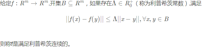
Lipschitz continuity

     Based on 1-Lipschitz continuity, the function, f, must satisfy the following property: 

     Furthermore, a real function, 𝑓: 𝑅 → 𝑅 , that satisfies the property is called K-Lipschitz continuous.
例子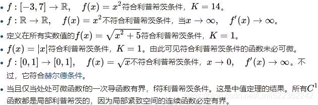

###########################

Using EM distance in practice for GANs

     Now, the question is, how do we find such a 1-Lipschitz continuous function to compute the Wasserstein distance between the distribution of real (𝑃𝑟) and fake (𝑃𝑔) outputs for a GAN? While the theoretical concepts behind the WGAN approach may seem complicated at first, the answer to this question is simpler than it may appear. Recall that we consider deep NNs to be universal function approximators. This means that we can simply train an NN model to approximate the Wasserstein distance function. As you saw in the previous section, the simple GAN uses a discriminator in the form of a classifier. For WGAN, the discriminator can be changed to behave as a critic, which returns a scalar score instead of a probability value. We can interpret this score as how realistic the input images are (like an art critic giving scores to artworks in a gallery).

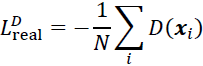
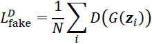
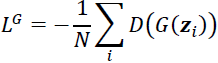
     To train a GAN using the Wasserstein distance, the losses for the discriminator, D, and generator, G, are defined as follows. The critic (that is, the discriminator network) returns its outputs for the batch of real image examples and the batch of synthesized examples. We use the notations D(x) and D(G(z)), respectively. Then, the following loss terms can be defined:

• • The real component of the discriminator's loss:
• • The fake component of the discriminator's loss:
• • The loss for the generator: 

     That will be all for the WGAN, except that we need to ensure that the 1-Lipschitz property of the critic function is preserved during training. For this purpose, the WGAN paper proposes clamping the weights to a small region, for example, [–0.01, 0.01].

Gradient penalty

     In the paper by Arjovsky et al., weight clipping is suggested for the 1-Lipschitz property of the discriminator (or critic). However, in another paper titled Improved Training of Wasserstein GANs, which is freely available at https://arxiv.org/pdf/1704.00028.pdf, Ishaan Gulrajani et al. showed that clipping the weights can lead to exploding and vanishing gradients. Furthermore, weight clipping can also lead to capacity underuse未充分利用, which means that the critic network is limited to learning only some simple functions, as opposed to more complex functions. Therefore, rather than clipping the weights, Ishaan Guljarani et al. proposed gradient penalty (GP) as an alternative solution. The result is the WGAN with gradient penalty (WGAN-GP).

The procedure for the GP that is added in each iteration can be summarized by the following sequence of steps:

• 1. For each pair of real and fake examples () in a given batch, choose a random number, , sampled from a uniform distribution, that is, ∈ 𝑈(0, 1).
• 2. Calculate an interpolation between the real and fake examples: , resulting in a batch of interpolated examples.
• 3. Compute the discriminator (critic) output for all the interpolated examples, .
• 4. Calculate the gradients of the critic's output with respect to each interpolated example, that is, .
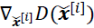• 5. Compute the GP as .
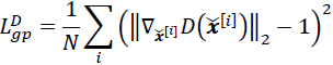  #  and 

The total loss for the discriminator is then as follows:  Here, 𝜆 is a tunable hyperparameter.

Implementing WGAN-GP to train the DCGAN model

     We will be making a few additional modifications to the DCGAN model in the remaining sections of this chapter. Note that the preprocess() function for transforming the dataset must change to output an image tensor instead of flattening the image to a vector. The following code shows the necessary modifications to build the dataset, as well as creating the new generator and discriminator networks:

mnist_bldr = tfds.builder('mnist')
mnist_bldr.download_and_prepare()
mnist = mnist_bldr.as_dataset( shuffle_files=False )

def preprocess( ex, mode='uniform' ):
  image = ex['image']
  # change the range of input pixel intensities to [0, 1]
  image = tf.image.convert_image_dtype( image, tf.float32 ) # /255.0 and tf.uint8 ==> tf.float32
  # scale them by a factor of 2 and shift them by –1 such that 
  # the pixel intensities will be rescaled to be in the range [–1, 1]
  image = image*2 -1.0

  if mode == 'uniform':
    input_z = tf.random.uniform( shape=(z_size,), minval=-1.0, maxval=1.0 )
  elif mode == 'normal':
    input_z = tf.random.normal( shape=(z_size,) ) # mean=0.0, stddev=1.0
  
  return input_z, image

     We have already defined the helper functions that create the generator and discriminator networks for DCGAN (make_dcgan_generator() and make_dcgan_discriminator()). The code to build the DCGAN model is as follows: 

num_epochs = 100
batch_size = 128
image_size = (28,28)
z_size = 20
mode_z = 'uniform'
lambda_gp  = 10.0

tf.random.set_seed(1)
np.random.seed(1)

## Set-up the dataset
mnist_trainset = mnist['train']
mnist_trainset = mnist_trainset.map( preprocess )

mnist_trainset = mnist_trainset.shuffle(10000)
mnist_trainset = mnist_trainset.batch( batch_size, drop_remainder=True )

## Set-up the model
with tf.device(device_name):
  gen_model = make_dcgan_generator()
  gen_model.build( input_shape=(None, z_size) )
  gen_model.summary()

  disc_model = make_dcgan_discriminator()
  disc_model.build( input_shape=(None, np.prod(image_size)) ) # 28*28*1
  disc_model.summary()

      Now we can train the model. Note that, typically, the RMSprop optimizer is recommended for WGAN (without the GP), whereas the Adam optimizer is used for WGAN-GP. The code is as follows:

import time

## optimizers:
g_optimizer = tf.keras.optimizers.Adam(0.0002)
d_optimizer = tf.keras.optimizers.Adam(0.0002)

######################## 𝒙̂ = 𝑔(𝒛) ########################
if mode_z == 'uniform':
  fixed_z = tf.random.uniform( shape=(batch_size, z_size),
                               minval=-1, maxval=1
            )
elif mode_z == 'normal':
  fixed_z = tf.random.normal( shape=(batch_size, z_size)
            )
  
def create_samples( g_model, input_z ):
  g_output = g_model( input_z, training=False ) # for freezing the generator
  images = tf.reshape( g_output,                # print( *image_size ) ==> 28 28
                                # (batch_size, image_size)  ==> ( 64, (28, 28) )                  
                       (batch_size, *image_size)          # ==> ( 64, 28, 28 )
                     ) 
  # since we scaled the pixel intensities by a factor of 2 and shift them by –1
  # such that the pixel intensities to be in the range [–1, 1] 
  return (images+1)/2.0

all_losses = []
epoch_samples = []

import time

start_time = time.time()

for epoch in range( 1, num_epochs+1 ):
  epoch_losses = []
  for i, (input_z, input_real) in enumerate( mnist_trainset ):
    ########## Compute discriminator's loss and gradients ##########
    with tf.GradientTape() as d_tape, tf.GradientTape() as g_tape:
      # gen_model = make_dcgan_generator()
      # input_z(batch_size, 20) ==> InputLayer
      # ==> Dense(6272) ==> (batch_size, 6272) ==> BatchNormalization ==> LeakyReLU
      # ==> Reshape     ==> (batch_size, 7,7,128)
      # ==> Conv2DTranspose ==> (batch_size, 7,7,128) ==> BatchNormalization ==> LeakyReLU
      # ==> Conv2DTranspose ==> (batch_size, 14,14,64) ==> BatchNormalization ==> LeakyReLU
      # ==> Conv2DTranspose ==> (batch_size, 28,28,32) ==> BatchNormalization ==> LeakyReLU
      # ==> Conv2DTranspose(activation='tanh') ==> (batch_size, 28,28,1) : Fake (synthesized) image
      g_output = gen_model( input_z, training=True )

      # disc_model = make_dcgan_discriminator()
      # (batch_size, 28,28,1) ==> InputLayer
      # ==> Conv2D ==> (batch_size,28,28,64) ==> BatchNormalization ==> LeakyReLU
      # ==> Conv2D ==> (batch_size,14,14,128)==> BatchNormalization ==> LeakyReLU ==> Dropout(0.3)
      # ==> Conv2D ==> (batch_size,7,7,256)  ==> BatchNormalization ==> LeakyReLU ==> Dropout(0.3)
      # ==> Conv2D ==> (batch_size,1,1,1)
      # ==> Reshape ==> (batch_size,1)
      d_critics_real = disc_model( input_real, training=True )
      d_critics_fake = disc_model( g_output, training=True )

      ########## Compute generator's loss ##########
      g_loss = -tf.math.reduce_mean( d_critics_fake )

      ########## Compute discriminator's losses ##########
      d_loss_real = -tf.math.reduce_mean( d_critics_real )
      d_loss_fake = tf.math.reduce_mean( d_critics_fake )
      d_loss = d_loss_real + d_loss_fake

      ########## Gradient penalty ##########
      with tf.GradientTape() as gp_tape:
        alpha = tf.random.uniform( shape=[d_critics_real.shape[0], 1,1,1],
                                   minval=0.0, maxval=1.0
                                 )
        interpolated = ( alpha*input_real + (1-alpha)*g_output )
        gp_tape.watch( interpolated ) # Ensures that tensor is being traced by this tape.

        d_critics_intp = disc_model(interpolated) # Compute the discriminator (critic) output for all the interpolated examples

      grads_intp = gp_tape.gradient( d_critics_intp, 
                                     [interpolated,] 
                                   )[0]

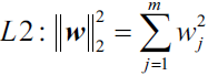
      grads_intp_l2 = tf.sqrt( tf.reduce_sum( tf.square(grads_intp), 
                                              axis=[1,2,3] # since image is 3D( w,h,c)
                                            ) # ==> 1D-list  
                             ) ##########
      
      D_L_gp = tf.reduce_mean( tf.square( grads_intp_l2 - 1.0 ) )
      d_loss = d_loss + lambda_gp * D_L_gp # d_loss_real + d_loss_fake + lambda*D_L_gp

    ########## Optimization: Compute the gradients apply them ##########
    d_grads = d_tape.gradient( d_loss, disc_model.trainable_variables )
                                 # List of (gradient, variable) pairs.
    d_optimizer.apply_gradients( grads_and_vars=zip( d_grads, 
                                                     disc_model.trainable_variables
                                                   )
                               )
    
    g_grads = g_tape.gradient( g_loss, gen_model.trainable_variables )
    g_optimizer.apply_gradients( grads_and_vars=zip( g_grads, 
                                                     gen_model.trainable_variables 
                                                   )
                               )
    epoch_losses.append( ( g_loss.numpy(), 
                           d_loss.numpy(),
                           d_loss_real.numpy(),
                           d_loss_fake.numpy()
                         )
                       )
    
  all_losses.append( epoch_losses ) # for each epoch

  print( 'Epoch {:-3d} | ET {:.2f} minutes | Avg Losses >> G/D {:6.2f}/{:6.2f}'\
        '\n\t\t\t\t\t[D-Real: {:6.2f}, D-Fake: {:6.2f}]'.format(
                                      epoch, 
                                      ( time.time()-start_time )/60,
                                      *list( np.mean( all_losses[-1], # the latest epoch
                                                      axis=0 
                                                    ) # mean of all batches the latest epoch
                                           )
                                                               )
       )
  
  epoch_samples.append( create_samples( gen_model, fixed_z ).numpy() )
  # next epoch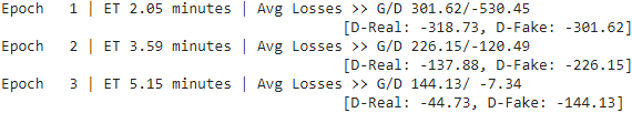

... ...

import pickle

pickle.dump({ 'all_losses': all_losses,
              'samples': epoch_samples
            },
            open('/content/drive/My Drive/Colab Notebooks/checkpoints/cp17-WDCGAN-learning.pkl',
                 'wb'
                )
            )

gen_model.save('/content/drive/My Drive/Colab Notebooks/models/cp17-WDCGAN-gan_generator.h5')
disc_model.save('/content/drive/My Drive/Colab Notebooks/models/cp17-WDCGAN-gan_discriminator.h5')

import itertools

fig = plt.figure( figsize=(12,10) )

#Plotting the losses
ax = fig.add_subplot(1,1,1)

# chain('ABC', 'DEF') --> A B C D E F
# *(( g_loss, d_loss, d_loss_real, d_loss_fake ),...)==>
# ( g_loss, d_loss, d_loss_real, d_loss_fake ), ...
# chain ==> iter( g_loss, d_loss, d_loss_real, d_loss_fake )

g_losses = [ item[0] for item in itertools.chain(*all_losses) ]
d_losses = [ item[1] for item in itertools.chain(*all_losses) ]

plt.plot( g_losses, label='Generator loss', alpha=0.95 )
plt.plot( d_losses, label='Discriminator loss', alpha=0.95 )
plt.legend( fontsize=20 )
ax.set_xlabel( 'Iteration', size=15 )
ax.set_ylabel( 'Loss', size=15 )
ax.set_ybound(upper=50000)

epochs = np.arange(1,101)
epoch2iter = lambda e: e*len( all_losses[-1] ) # all_losses[-1] : last epoch
epoch_ticks = [1,20,40,60,80,100]
newpos = [ epoch2iter(e) for e in epoch_ticks ]

ax2= ax.twiny()
ax2.set_xticks( newpos )
ax2.set_xticklabels( epoch_ticks )
ax2.xaxis.set_ticks_position( 'bottom' )
ax2.xaxis.set_label_position( 'bottom' )
# ax.spines[‘bottom’]获取底部的轴，通过set_position方法，设置底部轴的位置，
# outward:向绘图窗外
ax2.spines['bottom'].set_position( ('outward',60) )
ax2.set_xlabel( 'Epoch', size=15 )
ax2.set_xlim( ax.get_xlim() ) # Return the x-axis view limits.
ax.tick_params( axis='both', which='major', labelsize=15 )
ax2.tick_params( axis='both', which='major', labelsize=15 )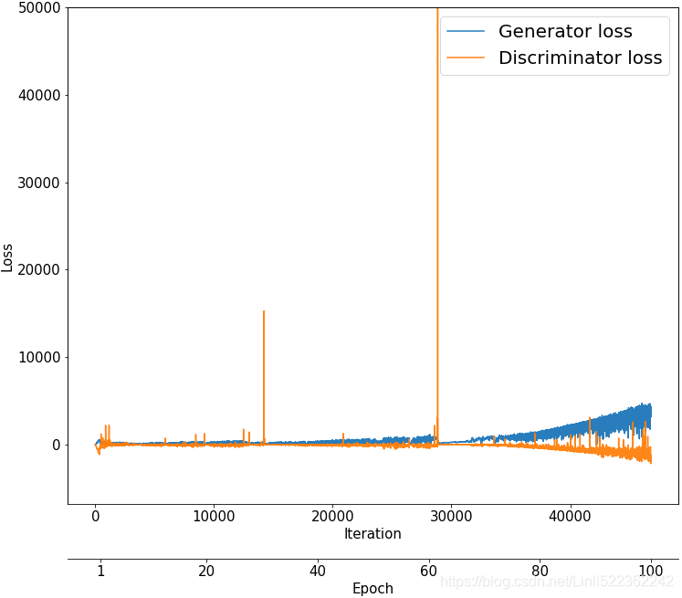

      Finally, let's visualize the saved examples at some epochs to see how the model is learning and how the quality of synthesized examples changes over the course of learning:

selected_epochs = [1,2,4,10,50,100]
fig = plt.figure( figsize=(10,14) )
for i, e in enumerate( selected_epochs ):
  for j in range(5):
    ax = fig.add_subplot( 6, 5, i*5+ j+1)
    ax.set_xticks([])
    ax.set_yticks([])

    if j==0:
      ax.text( -0.06, 0.5, #the anchor point of textbox(move to left by 0.06, move to up by 0.5)
               'Epoch {}'.format(e), rotation=90, size=18, color='red',
               horizontalalignment='right',#set the anchor point horizontal axis
               verticalalignment='center', #set the anchor point vertical axis
               transform=ax.transAxes )# move the anchor point to (-0.06, 0.5)
    image = epoch_samples[e-1][j]
    ax.imshow(image, cmap='gray_r')

plt.show()

The following figure shows the results:
 VS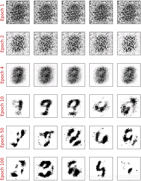 
     We used the same code to visualize the results as in the section on vanilla GAN(https://blog.csdn.net/Linli522362242/article/details/116565829). Comparing the new examples shows that DCGAN (with Wasserstein and GP) can generate images of a much higher quality.

Gan Mode collapse

     Due to the adversarial nature of GAN models, it is notoriously[noʊˈtɔːriəsli]臭名昭著 hard to train them. One common cause of failure in training GANs is when the generator gets stuck in a small subspace and learns to generate similar samples. This is called mode collapse, and an example is shown in the following figure.

     Besides the vanishing and exploding gradient problems that we saw previously, there are some further aspects that can also make training GAN models difficult (indeed, it is an art). Here are a few suggested tricks from GAN artists.

     One approach is called mini-batch discrimination, which is based on the fact that batches consisting of only real or fake examples are fed separately to the discriminator. In mini-batch discrimination, we let the discriminator compare examples across these batches to see whether a batch is real or fake. The diversity of a batch consisting of only real examples is most likely higher than the diversity of a fake batch if a model suffers from mode collapse.

     Another technique that is commonly used for stabilizing GAN training is feature matching. In feature matching, we make a slight modification to the objective function of the generator by adding an extra term that minimizes the difference between the original and synthesized images based on intermediate representations (feature maps) of the discriminator. We encourage you to read more about this technique in the original article by Ting-Chun Wang et al., titled High Resolution Image Synthesis and Semantic Manipulation with Conditional GANs, which is freely available at https://arxiv.org/pdf/1711.11585.pdf.

     During the training, a GAN model can also get stuck in several modes and just hop between them. To avoid this behavior, you can store some old examples and feed them to the discriminator to prevent the generator from revisiting previous modes. This technique is referred to as experience replay. Furthermore, you can train multiple GANs with different random seeds so that the combination of all of them covers a larger part of the data distribution than any single one of them.

Other GAN applications

     In this chapter, we mainly focused on generating examples using GANs and looked at a few tricks and techniques to improve the quality of synthesized outputs. The applications of GANs are expanding rapidly, including in computer vision, machine learning, and even other domains of science and engineering. A nice list of different GAN models and application areas can be found at https://github.com/hindupuravinash/the-gan-zoo.

     It is worth mentioning that we covered GANs in an unsupervised fashion, that is, no class label information was used in the models that were covered in this chapter. However, the GAN approach can be generalized to semi-supervised and supervised tasks, as well. For example, the conditional GAN (cGAN) proposed by Mehdi Mirza and Simon Osindero in the paper Conditional Generative Adversarial Nets (https://arxiv.org/pdf/1411.1784.pdf) uses the class label information and learns to synthesize new images conditioned on the provided label, that is, 𝒙̃ = 𝐺(𝒛|𝑦)—applied to MNIST. This allows us to generate different digits in the range 0-9 selectively. Furthermore, conditional GANs allows us to do image-to-image translation, which is to learn how to convert a given image from a specific domain to another. In this context, one interesting work is the Pix2Pix algorithm, published in the paper Image-to-Image Translation with Conditional Adversarial Networks by PhilipIsola et al.(https://arxiv.org/pdf/1611.07004.pdf). It is worth mentioning that in the Pix2Pix algorithm, the discriminator provides the real/fake predictions for multiple patches across the image as opposed to a single prediction for an entire image.

     CycleGAN is another interesting GAN model built on top of the cGAN, also for image-to-image translation. However, note that in CycleGAN, the training examples from the two domains are unpaired, meaning that there is no one-to-one correspondence between inputs and outputs. For example, using a CycleGAN, we could change the season of a picture taken in summer to winter. In the paper Unpaired Image-to-Image Translation Using Cycle-Consistent Adversarial Networks by Jun-Yan Zhu et al. (https://arxiv.org/pdf/1703.10593.pdf), an impressive example shows horses converted into zebras['zibrəz]斑马.

Summary

     In this chapter, you first learned about generative models in deep learning and their overall objective: synthesizing new data. We then covered how GAN models use a generator network and a discriminator network, which compete with each other in an adversarial training setting to improve each other. Next, we implemented a simple GAN model using only fully connected layers for both the generator and the discriminator.https://blog.csdn.net/Linli522362242/article/details/116565829

     We also covered how GAN models can be improved. First, you saw a DCGAN, which uses deep convolutional networks for both the generator and the discriminator. Along the way, you also learned about two new concepts: transposed convolution (for upsampling the spatial dimensionality of feature maps) and BatchNorm (for improving convergence during training). We then looked at a WGAN, which uses the EM distance to measure the distance between the distributions of real and fake samples. Finally, we talked about the WGAN with GP to maintain the 1-Lipschitz property instead of clipping the weights. In the next chapter, we will look at reinforcement learning, which is a completely different category of machine learning compared to what we have covered so far.