


Once you have a beautiful model that makes amazing predictions, what do you do with it? Well, you need to put it in production! This could be as simple as running the model on a batch of data and perhaps writing a script that runs this model every night. However, it is often much more involved. Various parts of your infrastructure may need to use this model on live data, in which case you probably want to wrap your model in a web service: this way, any part of your infrastructure can query your model at any time using a simple REST API (or some other protocol), as we discussed in Cp2(https://blog.csdn.net/Linli522362242/article/details/103387527). But as time passes, you need to regularly retrain your model on fresh data and push the updated version to production. You must handle model versioning, gracefully transition from one model to the next, possibly roll back to the previous model in case of problems, and perhaps run multiple different models in parallel to perform A/B experiments.(An A/B experiment consists in testing two different versions of your product on different subsets of users in order to check which version works best and get other insights.) If your product becomes successful, your service may start to get plenty of queries per second (QPS), and it must scale up to support the load. A great solution to scale up扩展 your service, as we will see in this chapter, is to use TF Serving, either on your own hardware infrastructure or via a cloud service such as Google Cloud AI Platform. It will take care of efficiently serving your model, handle graceful model transitions, and more. If you use the cloud platform, you will also get many extra features, such as powerful monitoring tools.
Moreover, if you have a lot of training data, and compute-intensive models, then training time may be prohibitively[proʊˈhɪbətɪvli]过分地 long. If your product needs to adapt to changes quickly, then a long training time can be a showstopper[ˈʃoʊˌstɑːpər]因特别精彩而被掌声打断的表演 (e.g., think of a news recommendation system promoting news from last week). Perhaps even more importantly, a long training time will prevent you from experimenting with new ideas. In Machine Learning (as in many other fields), it is hard to know in advance which ideas will work, so you should try out as many as possible, as fast as possible. One way to speed up training is to use hardware accelerators such as GPUs or TPUs. To go even faster, you can train a model across multiple machines, each equipped with multiple hardware accelerators. TensorFlow’s simple yet powerful Distribution Strategies API makes this easy, as we will see.
In this chapter we will look at how to deploy models, first to TF Serving, then to Google Cloud AI Platform. We will also take a quick look at deploying models to mobile apps, embedded devices, and web apps. Lastly, we will discuss how to speed up computations using GPUs and how to train models across multiple devices and servers using the Distribution Strategies API. That’s a lot of topics to discuss, so let’s get started!
Serving a TensorFlow Model
Once you have trained a TensorFlow model, you can easily use it in any Python code: if it’s a tf.keras model, just call its predict() method! But as your infrastructure grows, there comes a point where it is preferable to wrap your model in a small service whose sole role is to make predictions and have the rest of the infrastructure query it (e.g., via a REST or gRPC API).(A REST (or RESTful) API is an API that uses standard HTTP verbs, such as GET, POST, PUT, and DELETE, and uses JSON inputs and outputs. The gRPC protocol is more complex but more efficient. Data is exchanged using protocol buffers (see Cp13https://blog.csdn.net/Linli522362242/article/details/107704824).) This decouples[diːˈkʌpl] 使分离 your model from the rest of the infrastructure, making it possible to easily switch model versions or scale the service up as needed (independently from the rest of your infrastructure), perform A/B experiments, and ensure that all your software components rely on the same model versions. It also simplifies testing and development, and more. You could create your own microservice using any technology you want (e.g., using the Flask library), but why reinvent the wheel when you can just use TF Serving?
Using TensorFlow Serving
TF Serving is a very efficient, battle-tested model server that’s written in C++. It can sustain a high load, serve multiple versions of your models and watch a model repository to automatically deploy the latest versions, and more (see Figure 19-1). Figure 19-1. TF Serving can serve multiple models and automatically deploy the latest version of each model
So let’s suppose you have trained an MNIST model using tf.keras, and you want to deploy it to TF Serving. The first thing you have to do is export this model to Tensor‐Flow’s SavedModel format.
from tensorflow import keras
import numpy as np

(X_train_full, y_train_full), (X_test, y_test) = keras.datasets.mnist.load_data()
X_train_full = X_train_full[..., np.newaxis].astype(np.float32) / 255.
X_test = X_test[..., np.newaxis].astype( np.float32 )/255.
X_valid, X_train = X_train_full[:5000], X_train_full[5000:]
y_valid, y_train = y_train_full[:5000], y_train_full[5000:]
X_new = X_test[:3]
import tensorflow as tf
np.random.seed(42)
tf.random.set_seed(42)
model = keras.models.Sequential([
keras.layers.Flatten( input_shape=[28,28,1] ),
keras.layers.Dense(100, activation="relu"),
keras.layers.Dense(10, activation="softmax")
])
model.compile( loss="sparse_categorical_crossentropy",
optimizer = keras.optimizers.SGD(learning_rate=1e-2),
metrics = ["accuracy"]
)
model.fit( X_train, y_train, epochs=10, validation_data = (X_valid, y_valid) )
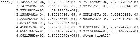
np.round( model.predict(X_new), 2 )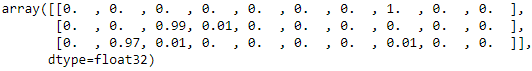
import os

model_version = "00001"
model_name = "my_mnist_model"
model_path = os.path.join( model_name, model_version )
model_path![]()
os.getcwd() ![]()
# https://www.jianshu.com/p/25358d2453cd
# !rm -rf {non-empty directory name} : delete everything in a non-empty directory
!rm -rf {model_name}![]() since this is a linux command
since this is a linux command
solution:
- os.remove('filename')
- os.rmdir('emptyDirectory')
- os.removedirs( 'emptyMultiLevelDirectories' )
- import shutil ==> shutil.rmtree('MultiLevelDirectories')
import shutil

shutil.rmtree( model_name )
Exporting SavedModels
TensorFlow provides a simple tf.saved_model.save() function to export models to the SavedModel format. All you need to do is give it the model, specifying its name and version number, and the function will save the model’s computation graph and its weights:
tf.saved_model.save( model, model_path )
If your warning is : 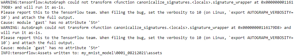
solution: if you are using tensorflow 2.1.1
pip install gast==0.2.2https://blog.csdn.net/Linli522362242/article/details/108037567
pip install tensorflow-serving-api==2.1.0will automally install tensorboard 2.1.0
Alternatively, you can just use the model’s save() method (model.save(model_path)): as long as the file’s extension is not .h5, the model will be saved using the SavedModel format instead of the HDF5 format.
It’s usually a good idea to include all the preprocessing layers in the final model you export so that it can ingest[ɪnˈdʒest]vt. 摄取 data in its natural form once it is deployed to production. This avoids having to take care of preprocessing separately within the application that uses the model. Bundling the preprocessing steps within the model also makes it simpler to update them later on and limits the risk of mismatch between a model and the preprocessing steps it requires.
Since a SavedModel saves the computation graph, it can only be used with models that are based exclusively on TensorFlow operations,
- excluding the tf.py_function() operation (which wraps arbitrary Python code). It also
- excludes dynamic tf.keras models (see Appendix G), since these models cannot be converted to computation graphs. Dynamic models need to be served using other tools (e.g., Flask).
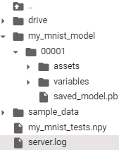
A SavedModel represents a version of your model. It is stored as a directory containing
- a saved_model.pb file, which defines the computation graph (represented as a serialized protocol buffer), and
- a variables subdirectory containing the variable values. For models containing a large number of weights, these variable values may be split across multiple files.
- A SavedModel also includes an assets subdirectory that may contain additional data, such as vocabulary files, class names, or some example instances for this model.
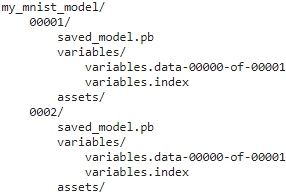
The directory structure is as follows (in this example, we don’t use assets):
for root, dirs, files in os.walk( model_name, topdown=True ):
    indent = '    ' * root.count( os.sep )
    print( '{}{}/'.format( indent, os.path.basename(root) ) )
    for filename in files:
        print( '{}{}'.format( indent + '    ', filename ) )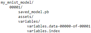
As you might expect, you can load a SavedModel using the tf.saved_model.load() function. However, the returned object is not a Keras model: it represents the Saved‐Model, including its computation graph and variable values. You can use it like a function, and it will make predictions (make sure to pass the inputs as tensors of the appropriate type):
saved_model = tf.saved_model.load(model_path)
y_pred = saved_model(tf.constant(X_new, dtype=tf.float32))
Alternatively, you can load this SavedModel directly to a Keras model using the keras.models.load_model() function:
model = keras.models.load_model(model_path)
y_pred = model.predict(tf.constant(X_new, dtype=tf.float32))
TensorFlow also comes with a small saved_model_cli command-line tool to inspect SavedModels:
!saved_model_cli show --dir {model_path}The given SavedModel contains the following tag-sets:
serve
!saved_model_cli show --dir {model_path} --tag_set serveThe given SavedModel MetaGraphDef contains SignatureDefs with the following keys:
SignatureDef key: "__saved_model_init_op"
SignatureDef key: "serving_default
!saved_model_cli show --dir {model_path} --tag_set serve \
                      --signature_def serving_default
The given SavedModel SignatureDef contains the following input(s):
inputs['flatten_1_input'] tensor_info:
dtype: DT_FLOAT
shape: (-1, 28, 28, 1)
name: serving_default_flatten_1_input:0
The given SavedModel SignatureDef contains the following output(s):
outputs['dense_3'] tensor_info:
dtype: DT_FLOAT
shape: (-1, 10)
name: StatefulPartitionedCall:0
Method name is: tensorflow/serving/predict
A SavedModel contains one or more metagraphs元图. A metagraph is a computation graph plus some function signature definitions (including their input and output names, types, and shapes). Each metagraph is identified by a set of tags. For example, you may want to have
- a metagraph containing the full computation graph, including the training operations (this one may be tagged "train", for example), and
- another metagraph containing a pruned computation graph with only the prediction operations, including some GPU-specific operations (this metagraph may be tagged "serve", "gpu").
However, when you pass a tf.keras model to the tf.saved_model.save() function, by default the function saves a much simpler SavedModel: it saves a single metagraph tagged "serve", which contains two signature definitions,
- an initialization function (called __saved_model_init_op, which you do not need to worry about) and
- a default serving function (called serving_default). When saving a tf.keras model, the default serving function corresponds to the model’s call() function, which of course makes predictions.
!saved_model_cli show --dir {model_path} --allMetaGraphDef with tag-set: 'serve' contains the following SignatureDefs:
signature_def['__saved_model_init_op']:
The given SavedModel SignatureDef contains the following input(s):
The given SavedModel SignatureDef contains the following output(s):
outputs['__saved_model_init_op'] tensor_info:
dtype: DT_INVALID
shape: unknown_rank
name: NoOp
Method name is:
signature_def['serving_default']:
The given SavedModel SignatureDef contains the following input(s):
inputs['flatten_1_input'] tensor_info:
dtype: DT_FLOAT
shape: (-1, 28, 28, 1)
name: serving_default_flatten_1_input:0
The given SavedModel SignatureDef contains the following output(s):
outputs['dense_3'] tensor_info:
dtype: DT_FLOAT
shape: (-1, 10)
name: StatefulPartitionedCall:0
Method name is: tensorflow/serving/predict
Defined Functions:
Function Name: '__call__'
Option #1
Callable with:
Argument #1
flatten_1_input: TensorSpec(shape=(None, 28, 28, 1), dtype=tf.float32, name='flatten_1_input')
Argument #2
DType: bool
Value: True
Argument #3
DType: NoneType
Value: None
Option #2
Callable with:
Argument #1
inputs: TensorSpec(shape=(None, 28, 28, 1), dtype=tf.float32, name='inputs')
Argument #2
DType: bool
Value: True
Argument #3
DType: NoneType
Value: None
Option #3
Callable with:
Argument #1
inputs: TensorSpec(shape=(None, 28, 28, 1), dtype=tf.float32, name='inputs')
Argument #2
DType: bool
Value: False
Argument #3
DType: NoneType
Value: None
Option #4
Callable with:
Argument #1
flatten_1_input: TensorSpec(shape=(None, 28, 28, 1), dtype=tf.float32, name='flatten_1_input')
Argument #2
DType: bool
Value: False
Argument #3
DType: NoneType
Value: None
Function Name: '_default_save_signature'
Option #1
Callable with:
Argument #1
flatten_1_input: TensorSpec(shape=(None, 28, 28, 1), dtype=tf.float32, name='flatten_1_input')
Function Name: 'call_and_return_all_conditional_losses'
Option #1
Callable with:
Argument #1
inputs: TensorSpec(shape=(None, 28, 28, 1), dtype=tf.float32, name='inputs')
Argument #2
DType: bool
Value: False
Argument #3
DType: NoneType
Value: None
Option #2
Callable with:
Argument #1
inputs: TensorSpec(shape=(None, 28, 28, 1), dtype=tf.float32, name='inputs')
Argument #2
DType: bool
Value: True
Argument #3
DType: NoneType
Value: None
Option #3
Callable with:
Argument #1
flatten_1_input: TensorSpec(shape=(None, 28, 28, 1), dtype=tf.float32, name='flatten_1_input')
Argument #2
DType: bool
Value: True
Argument #3
DType: NoneType
Value: None
Option #4
Callable with:
Argument #1
flatten_1_input: TensorSpec(shape=(None, 28, 28, 1), dtype=tf.float32, name='flatten_1_input')
Argument #2
DType: bool
Value: False
Argument #3
DType: NoneType
Value: None

The saved_model_cli tool can also be used to make predictions (for testing, not really for production). Suppose you have a NumPy array (X_new) containing three images of handwritten digits that you want to make predictions for. You first need to export them to NumPy’s npy format:
np.save( "my_mnist_tests.npy", X_new )input_name = model.input_names[0]
input_name![]()
And now let's use saved_model_cli to make predictions for the instances we just saved:
!saved_model_cli run --dir {model_path} --tag_set serve \
                     --signature_def serving_default    \
                     --inputs {input_name}=my_mnist_tests.npy
np.round([ [1.0555653e-04, 1.6835124e-07, 7.0605183e-04, 2.1929101e-03, 2.6903028e-06,
            7.4441166e-05, 3.1963769e-08, 9.9645138e-01, 4.2528231e-05, 4.2422040e-04,
           ],
           [8.3398668e-04, 2.8253320e-05, 9.8908687e-01, 7.4617229e-03, 8.6197012e-08,
            2.1671386e-04, 1.5678996e-03, 9.6067954e-10, 8.0423383e-04, 8.4014978e-08,
           ],
           [5.5251930e-05, 9.7237802e-01, 8.7161232e-03, 2.1327569e-03, 4.6825167e-04,
            2.8200611e-03, 2.1204432e-03, 6.9332127e-03, 4.0979674e-03, 2.7782060e-04,
           ]
         ],
         2
        )
Installing TensorFlow Serving
There are many ways to install TF Serving: using a Docker image, (If you are not familiar with Docker, it allows you to easily download a set of applications packaged in a Docker image (including all their dependencies and usually some good default configuration) and then run them on your system using a Docker engine. When you run an image, the engine creates a Docker container that keeps the applications well isolated from your own system (but you can give it some limited access if you want). It is similar to a virtual machine, but much faster and more lightweight, as the container relies directly on the host’s kernel. This means that the image does not need to include or run its own kernel.) using the system’s package manager, installing from source, and more. Let’s use the Docker option, which is highly recommended by the TensorFlow team as it is simple to install, it will not mess with your system, and it offers high performance. You
- first need to install Docker.
- Then download the official TF Serving Docker image
Install Docker if you don't have it already. Then run:
docker pull tensorflow/serving

export ML_PATH=$HOME/ml # or wherever this project is
docker run -it --rm -p 8500:8500 -p 8501:8501 \
   -v "$ML_PATH/my_mnist_model:/models/my_mnist_model" \
   -e MODEL_NAME=my_mnist_model \
   tensorflow/serving
Once you are finished using it, press Ctrl-C to shut down the server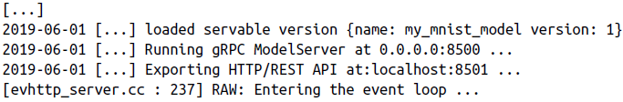
That’s it! TF Serving is running. It loaded our MNIST model (version 1), and it is serving it through both gRPC (on port 8500) and REST (on port 8501). Here is what all the command-line options mean:
- -it
Makes the container interactive (so you can press Ctrl-C to stop it) and displays the server’s output.
- --rm
Deletes the container when you stop it (no need to clutter your machine with interrupted containers). However, it does not delete the image.
- -p 8500:8500
Makes the Docker engine forward the host’s TCP port 8500 to the container’s TCP port 8500. By default, TF Serving uses this port to serve the gRPC API.
- -p 8501:8501
Forwards the host’s TCP port 8501 to the container’s TCP port 8501. By default, TF Serving uses this port to serve the REST API.
- -v "$ML_PATH/my_mnist_model:/models/my_mnist_model"
Makes the host’s $ML_PATH/my_mnist_model directory available to the container at the path /models/mnist_model. On Windows, you may need to replace / with \ in the host path (but not in the container path).
- -e MODEL_NAME=my_mnist_model
Sets the container’s MODEL_NAME environment variable, so TF Serving knows which model to serve. By default, it will look for models in the /models directory, and it will automatically serve the latest version it finds.
- tensorflow/serving
This is the name of the image to run.
In google colab:
tensorflow_model_server
import sys
assert sys.version_info >= (3, 5)

# Is this notebook running on Colab or Kaggle?
IS_COLAB = "google.colab" in sys.modules
IS_KAGGLE = "kaggle_secrets" in sys.modules

if IS_COLAB or IS_KAGGLE:
    !echo "deb http://storage.googleapis.com/tensorflow-serving-apt stable tensorflow-model-server tensorflow-model-server-universal" > /etc/apt/sources.list.d/tensorflow-serving.list
    !curl https://storage.googleapis.com/tensorflow-serving-apt/tensorflow-serving.release.pub.gpg | apt-key add -
    !apt update && apt-get install -y tensorflow-model-server
    !pip install -q -U tensorflow-serving-api
# First lets update all the packages to the latest ones with the following command.
!sudo apt update
# Now we want to install some prerequisite packages which will let us use HTTPS over apt.
!sudo apt install apt-transport-https ca-certificates curl software-properties-common
# After that we will add the GPG key for the official Docker repository to the system.
!curl -fsSL https://download.docker.com/linux/ubuntu/gpg | sudo apt-key add -
# We will need to add the Docker repository to our APT sources:
!sudo add-apt-repository "deb [arch=amd64] https://download.docker.com/linux/ubuntu bionic stable"
# Next lets update the package database with our newly added Docker package repo.
!sudo apt update
...
# Finally lets install docker with the below command:
!sudo apt install docker
# model_path                                  # my_mnist_model/00001
# os.path.abspath(model_path)                 # /content/my_mnist_model/00001
# os.path.split(os.path.abspath(model_path))  # ('/content/my_mnist_model', '00001')
os.path.split(os.path.abspath(model_path))[0] # /content/my_mnist_model![]()
os.getcwd() Alternatively, if tensorflow_model_server is installed (e.g., if you are running this notebook in Colab), then the following 3 cells will start the server:
os.environ["MODEL_DIR"] = os.path.split(os.path.abspath(model_path))[0]![]()
%%bash --bg
nohup tensorflow_model_server \
     --rest_api_port=8501 \
     --model_name=my_mnist_model \
--model_base_path="${MODEL_DIR}" >server.log 2>&1![]()
- %% bash 前台、后台(back ground)作业的切换、执行可使用内建命令fg、bg。
- nohup https://baike.baidu.com/item/nohup/5683841?fr=aladdin
就是不挂断的意思( no hang up)
该命令的一般形式为:nohup command & OR nohup Command [ Arg ... ] [ & ] - tensorflow_model_serving
This is the name of the image to run. - --rest_api_port=8501
Forwards the host’s TCP port 8501 to the container’s TCP port 8501. By default,
TF Serving uses this port to serve the REST API. - --model_name=my_mnist_model
Sets the container’s MODEL_NAME environment variable, so TF Serving knows
which model to serve. By default, it will look for models in the /models directory,
and it will automatically serve the latest version it finds. -
--model_base_path="${MODEL_DIR}"
make the container model base path at the path /content/my_mnist_model -
如果使用nohup命令提交作业,那么在缺省情况下该作业的所有输出都被重定向到一个名为nohup.out的文件中,除非另外指定了输出文件:
nohup command > server.log 2>&1
-
在上面的例子中, 0 – stdin (standard input),1 – stdout (standard output),2 – stderr (standard error) ;
2>&1是将标准错误(2)重定向到标准输出(&1),
标准输出(&1)再被重定向输入到server.log文件中。!tail server.log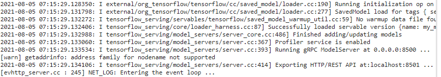
Querying TF Serving through the REST API
Let’s start by creating the query. It must contain the name of the function signature you want to call, and of course the input data:
import json

input_data_json = json.dumps( { "signature_name": "serving_default",
                                "instances": X_new.tolist()
                              }
                            )
Note that the JSON format is 100% text-based, so the X_new NumPy array had to be converted to a Python list and then formatted as JSON:
input_data_json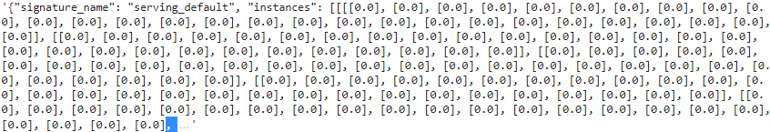
# python中str()与repr()函数的区别
# https://blog.csdn.net/xc_zhou/article/details/80952314
repr( input_data_json )[:1500] + "..." 
Now let’s send the input data to TF Serving by sending an HTTP POST request. This can be done easily using the requests library (it is not part of Python’s standard library, so you will need to install it first, e.g., using pip):
!pip install requests
Now let's use TensorFlow Serving's REST API to make predictions:
import requests

SERVER_URL = 'http://localhost:8501/v1/models/my_mnist_model:predict'
response = requests.post( SERVER_URL, data = input_data_json )
response.raise_for_status() # raise an exception in case of error
response = response.json()
The response is a dictionary containing a single "predictions" key. The corresponding value is the list of predictions. This list is a Python list, so let’s convert it to a NumPy array and round the floats it contains to the second decimal:
y_proba = np.array( response['predictions'] )
y_proba.round(2) ![]()
Hurray, we have the predictions! The model
- is close to 100% confident that the 1st image is a 7 (image_class: digit 7),
- 99% confident that the second image is a 2 (image_class: digit 2), and
- 97% confident that the third image is a 1(image_class: digit 1).
The REST API is nice and simple, and it works well when the input and output data are not too large. Moreover, just about any client application can make REST queries without additional dependencies, whereas other protocols are not always so readily available. However, it is based on JSON, which is text-based and fairly verbose. For example, we had to convert the NumPy array to a Python list, and every float ended up represented as a string. This is very inefficient, both in terms of serialization/deserialization time (to convert all the floats to strings and back) and in terms of payload size: many floats end up being represented using over 15 characters, which translates to over 120 bits for 32-bit floats! This will result in high latency and bandwidth usage when transferring large NumPy arrays.(To be fair, this can be mitigated by serializing the data first and encoding it to Base64 before creating the REST request. Moreover, REST requests can be compressed using gzip, which reduces the payload size significantly.) So let’s use gRPC instead.
When transferring large amounts of data, it is much better to use the gRPC API (if the client supports it), as it is based on a compact binary format and an efficient communication protocol (based on HTTP/2 framing).
Querying TF Serving through the gRPC API
The gRPC API expects a serialized PredictRequest protocol buffer as input, and it outputs a serialized PredictResponse protocol buffer. These protobufs are part of the tensorflow-serving-api library, which you must install (e.g., using pip). First, let’s create the request:
The following code creates a PredictRequest protocol buffer and fills in the required fields, including
- the model name (defined earlier),
- the signature name of the function we want to call, and finally
- the input data, in the form of a Tensor protocol buffer.
- The tf.make_tensor_proto() function creates a Tensor protocol buffer based on the given tensor or NumPy array, in this case X_new.
from tensorflow_serving.apis.predict_pb2 import PredictRequest

# https://tensorflow.google.cn/versions/r2.1/api_docs/python/tf/make_tensor_proto
# https://www.w3cschool.cn/tensorflow_python/tensorflow_python-fxrl2fa6.html
request = PredictRequest()
request.model_spec.name = model_name                  # 'my_mnist_model'
request.model_spec.signature_name = 'serving_default'
input_name = model.input_names[0]                     # 'flatten_input'

request.inputs[input_name].CopyFrom( tf.make_tensor_proto(X_new) ) # X_new.shape ==> (3, 28, 28, 1)
Next, we’ll send the request to the server and get its response (for this you will need the grpcio library, which you can install using pip):
The following code is quite straightforward: after the imports, we
- create a gRPC communication channel to localhost on TCP port 8500, then
- we create a gRPC service over this channel and use it to send a request, with a 10-second timeout (not that the call is synchronous: it will block until it receives the response or the timeout period expires).
In this example the channel is insecure (no encryption, no authentication), but gRPC and TensorFlow Serving also support secure channels over SSL/TLS.
import grpc
from tensorflow_serving.apis import prediction_service_pb2_grpc

channel = grpc.insecure_channel( 'localhost:8500' )
predict_service = prediction_service_pb2_grpc.PredictionServiceStub( channel )
response = predict_service.Predict( request, timeout=10.0 )response# y_proba
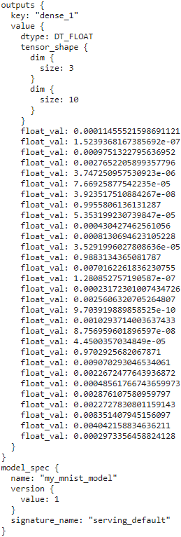
Next, let’s convert the PredictResponse protocol buffer to a tensor:
output_name = model.output_names[0] # model.output_names : ['dense_1']
outputs_proto = response.outputs[output_name] # key='dense_1': value
y_proba = tf.make_ndarray( outputs_proto )
y_proba.round(2)
If you run this code and print y_proba.numpy().round(2), you will get the exact same estimated class probabilities as earlier. And that’s all there is to it: in just a few lines of code, you can now access your TensorFlow model remotely, using either REST or gRPC.
output_name = model.output_names[0]
outputs_proto = response.outputs[output_name]
shape = [ dim.size for dim in outputs_proto.tensor_shape.dim ] # [3, 10]
y_proba = np.array( outputs_proto.float_val ).reshape( shape )
y_proba.round(2)![]()
Deploying a new model version
Now let’s create a new model version and export a SavedModel to the my_mnist_model/0002 directory, just like earlier:
np.random.seed(42)
tf.random.set_seed(42)

model = keras.models.Sequential([
                                 keras.layers.Flatten( input_shape=[28,28,1] ),
                                 keras.layers.Dense( 50, activation="relu" ),
                                 keras.layers.Dense( 50, activation="relu" ),
                                 keras.layers.Dense( 10, activation="softmax" )
                                ])

model.compile( loss="sparse_categorical_crossentropy",
               optimizer = keras.optimizers.SGD( learning_rate=1e-2),
               metrics = ["accuracy"]
             )

history = model.fit( X_train, y_train, epochs=10,
                     validation_data=(X_valid, y_valid)
                   )
model_version = "0002"
model_name = "my_mnist_model"
model_path = os.path.join( 'drive/MyDrive/Colab Notebooks/', model_name, model_version )
model_path ![]()
tf.saved_model.save( model, model_path )
for root, dirs, files in os.walk( 'drive/MyDrive/Colab Notebooks/' + model_name ):
  # print(root.count( os.sep )) ==> 3 for 'my_mnist_model/' since 3 '/' before it
  indent = '    ' * (root.count( os.sep )-3)
  print( '{}{}/'.format( indent,
                         os.path.basename(root)
                       )
       )

  for filename in files:
    print( '{}{}'.format( indent + '    ',
                          filename
                        )
         )
OR https://blog.csdn.net/Linli522362242/article/details/110155280
from pathlib import Path

#Path(os.getcwd()) ==> Path(os.getcwd()) ==> PosixPath('/content')
path=Path( os.getcwd() )/'drive/MyDrive/Colab Notebooks'/model_name
path![]()
for root, dirs, files in os.walk( path ):
  #print(root.count( os.sep ))# ==> 5 for 'my_mnist_model/' since 5 '/' before it
  indent = '    ' * (root.count( os.sep )-5)
  print( '{}{}/'.format( indent,
                         os.path.basename(root)
                       )
       )

  for filename in files:
    print( '{}{}'.format( indent + '    ',
                          filename
                        )
         )
Warning: You may need to wait a minute before the new model is loaded by TensorFlow Serving.
- Querying TF Serving through the REST API
import requests

SERVER_URL = 'http://localhost:8501/v1/models/my_mnist_model:predict'
# import json

# input_data_json = json.dumps( { "signature_name": "serving_default",
#                                 "instances": X_new.tolist()
#                               }
#                             )
response = requests.post( SERVER_URL, data=input_data_json )
response.raise_for_status()
response = response.json()

response.keys()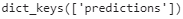
y_proba = np.array( response['predictions'] )
y_proba.round(2)
VS (previous version)
- Querying TF Serving through the gRPC API
from tensorflow_serving.apis.predict_pb2 import PredictRequest

# https://tensorflow.google.cn/versions/r2.1/api_docs/python/tf/make_tensor_proto
# https://www.w3cschool.cn/tensorflow_python/tensorflow_python-fxrl2fa6.html
request = PredictRequest()
request.model_spec.name = model_name                  # 'my_mnist_model'
request.model_spec.signature_name = 'serving_default'
input_name = model.input_names[0]                     # 'flatten_input'

request.inputs[input_name].CopyFrom( tf.make_tensor_proto(X_new) ) # X_new.shape ==> (3, 28, 28, 1)

import grpc
from tensorflow_serving.apis import prediction_service_pb2_grpc

channel = grpc.insecure_channel( 'localhost:8500' )
predict_service = prediction_service_pb2_grpc.PredictionServiceStub( channel )
response = predict_service.Predict( request, timeout=10.0 )

output_name = model.output_names[0] # model.output_names : ['dense_1']
outputs_proto = response.outputs[output_name] # key='dense_1': value
y_proba = tf.make_ndarray( outputs_proto )
y_proba.round(2)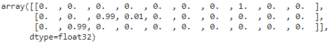
At regular intervals (the delay is configurable), TensorFlow Serving checks for new model versions. If it finds one, it will automatically handle the transition gracefully: by default, it will answer pending requests (if any) with the previous model version, while handling new requests with the new version.(If the SavedModel contains some example instances in the assets/extra directory, you can configure TF Serving to execute the model on these instances before starting to serve new requests with it. This is called model warmup: it will ensure that everything is properly loaded, avoiding long response times for the first requests.) As soon as every pending request has been answered, the previous model version is unloaded. You can see this at work in the TensorFlow Serving logs:
![]()
 This approach offers a smooth transition, but it may use too much RAM (especially GPU RAM, which is generally the most limited). In this case, you can configure TF Serving so that it
- handles all pending requests with the previous model version and unloads it before loading and using the new model version. This configuration will
- avoid having two model versions loaded at the same time, but the service will be unavailable for a short period.
As you can see, TF Serving makes it quite simple to deploy new models. Moreover, if you discover that version 2 does not work as well as you expected, then rolling back to version 1 is as simple as removing the my_mnist_model/0002 directory
Another great feature of TF Serving is its automatic batching capability, which you can activate using the --enable_batching option upon startup. When TF Serving receives multiple requests within a short period of time (the delay is configurable), it will automatically batch them together before using the model. This offers a significant performance boost by leveraging the power of the GPU. Once the model returns the predictions, TF Serving dispatches each prediction to the right client. You can trade a bit of latency for a greater throughput by increasing the batching delay (see the --batching_parameters_file option). 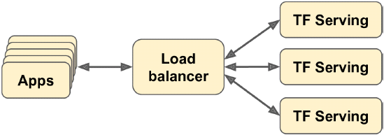
Figure 19-2. Scaling up TF Serving with load balancing
If you expect to get many queries per second, you will want to deploy TF Serving on multiple servers and load-balance the queries (see Figure 19-2). This will require deploying and managing many TF Serving containers across these servers. One way to handle that is to use a tool such as Kubernetes, which is an open source system for simplifying container orchestration across many servers. If you do not want to purchase, maintain, and upgrade all the hardware infrastructure, you will want to use virtual machines on a cloud platform such as Amazon AWS, Microsoft Azure, Google Cloud Platform, IBM Cloud, Alibaba Cloud, Oracle Cloud, or some other Platformas-a-Service (PaaS). Managing all the virtual machines, handling container orchestration[ˌɔːrkɪˈstreɪʃn]编排 (even with the help of Kubernetes), taking care of TF Serving configuration, tuning and monitoring—all of this can be a full-time job. Fortunately, some service providers can take care of all this for you. In this chapter we will use Google Cloud AI Platform because it’s the only platform with TPUs today, it supports TensorFlow 2, it offers a nice suite of AI services (e.g., AutoML, Vision API, Natural Language API), and it is the one I have the most experience with. But there are several other providers in this space, such as Amazon AWS SageMaker and Microsoft AI Platform, which are also capable of serving TensorFlow models.
Now let’s see how to serve our wonderful MNIST model on the cloud!
Creating a Prediction Service on GCP AI Platform
Before you can deploy a model, there’s a little bit of setup to take care of:
- 1. Log in to your Google account, and then go to the Google Cloud Platform (GCP) console (see Figure 19-3). If you don’t have a Google account, you’ll have to create one.

- 2. If it is your first time using GCP, you will have to read and accept the terms and conditions. Click Tour Console if you want. At the time of this writing, new users are offered a free trial, including $300 worth of GCP credit that you can use over the course of 91 days. You will only need a small portion of that to pay for the services you will use in this chapter. Upon signing up for the free trial, you will still need to create a payment profile and enter your credit card number: it is used for verification purposes (probably to avoid people using the free trial multiple times), but you will not be billed. Activate and upgrade your account if requested.

- 3. If you have used GCP before and your free trial has expired, then the services you will use in this chapter will cost you some money. It should not be too much, especially if you remember to turn off the services when you do not need them anymore. Make sure you understand and agree to the pricing conditions before you run any service. I hereby decline any responsibility if services end up costing more than you expected! Also make sure your billing account is active. To check, open the navigation menu on the left and click Billing, and make sure you have set up a payment method and that the billing account is active.

- 4. Every resource in GCP belongs to a project. This includes all the virtual machines you may use, the files you store, and the training jobs you run. When you create an account, GCP automatically creates a project for you, called “My First Project.” If you want, you can change its display name by going to the project settings: in the navigation menu (on the left of the screen), select IAM & admin → Settings,
 ==>
==>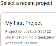
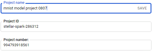
change the project’s display name, and click Save. Note that the project also has a unique ID and number. You can choose the project ID when you create a project, but you cannot change it later. The project number is automatically generated and cannot be changed.
If you want to create a new project, click the CREATE PROJECT at the top-right of the page,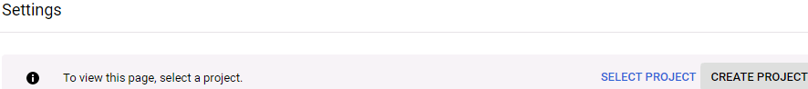 then type the Project name and enter the Project ID. Make sure billing is active for this new project.
Always set an alarm to remind yourself to turn services off when you know you will only need them for a few hours, or else you might leave them running for days or months, incurring potentially significant costs.
- 5. Now that you have a GCP account with billing activated, you can start using the services. The first one you will need is Google Cloud Storage (GCS): this is where you will put the SavedModels, the training data, and more. In the navigation menu, scroll down to the Storage section, and click Cloud Storage → Browser.

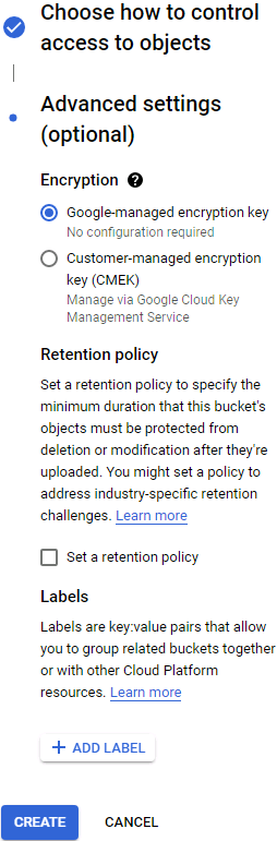
All your files will go in one or more buckets. Click Create Bucket and choose the bucket name (you may need to activate the Storage API first==> APIs & Services ==> Library ).==> Select a Project ==>
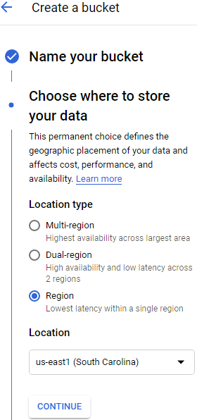
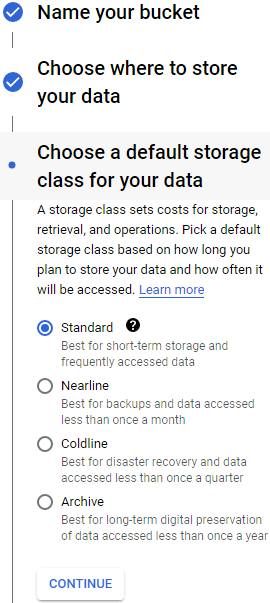
 GCS uses a single worldwide namespace for buckets, so simple names like “machine-learning” will most likely not be available. Make sure the bucket name conforms to DNS naming conventions, as it may be used in DNS records. Moreover, bucket names are public, so do not put anything private in there. It is common to use your domain name or your company name as a prefix to ensure uniqueness, or simply use a random number as part of the name. Choose the location where you want the bucket to be hosted, and the rest of the options should be fine by default. Then click Create.
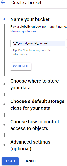 ==>
==> ==>
==> ==>
==> ==>
==>
- 6. Upload the my_mnist_model folder you created earlier (including one or more versions) to your bucket. To do this, just go to the GCS(Google Cloud Storage) Browser, click the bucket, then drag and drop the my_mnist_model folder from your system to the bucket (see Figure 19-4).
Alternatively, you can click “Upload folder” and select the my_mnist_model folder to upload. By default, the maximum size for a SavedModel is 250 MB, but it is possible to request a higher quota.
Figure 19-4. Uploading a SavedModel to Google Cloud Storage ==>
==>
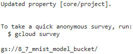
Project ID: stellar-spark-286312
Connecting to GCS bucket
Once your bucket is set up you can connect Colab to GCS using Google Auth API and gsutil.
First you need to authenticate yourself in the same way you did for Google Drive,
then you need to set your project ID before you can access your bucket(s). The project ID is shown in the Resource Manager or the URL when you manage your buckets. -
from google.colab import auth

auth.authenticate_user()

project_id = 'stellar-spark-286312'
!gcloud config set project {project_id}
!gsutil ls
This will connect to your project and list all buckets.
Next you can copy data from or to GCS usinggsutil cpcommand. Note that the content of your Google Drive is not under/content/drivedirectly, but in the subfolderMy Drive. If you copy more than a few files, use the-moption for gsutil, as it will enable multi-threading and speed up the copy process significantly.
https://cloud.google.com/storage/docs/gsutil/commands/cp
If you have a large number of files to transfer, you can perform a parallel multi-threaded/multi-processing copy using the top-level gsutil-moption (see gsutil help options):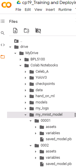 ==>
==>
bucket_name = '8_7_mnist_model_bucket'

!gsutil -m cp -r /content/drive/My\ Drive/Colab\ Notebooks/my_mnist_model gs://{bucket_name}
- 7. Now you need to configure AI Platform (formerly known as ML Engine) so that it knows which models and versions you want to use. In the navigation menu, scroll down to the Artificial Intelligence section, and click AI Platform → Models. Click Activate API (it takes a few minutes), then click “Create model.” Fill in the model details (see Figure 19-5) and click Create.
 ==>
==>
 >
>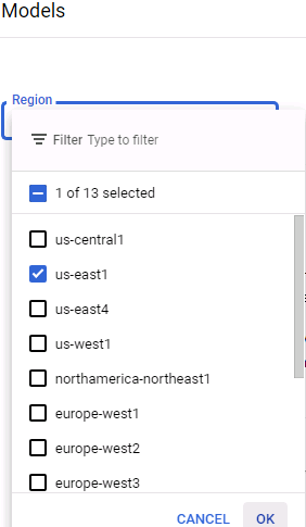


Figure 19-5. Creating a new model on Google Cloud AI Platform
-
8. Now that you have a model on AI Platform, you need to create a model version. In the list of models, click the model you just created, then click “Create version” and fill in the version details (see Figure 19-6): set the name, description, Python version (3.5 or above), framework (TensorFlow), framework version (2.0 if available, or 1.13),6 ML runtime version (2.0, if available or 1.13), machine type (choose “Single core CPU” for now), model path on GCS (this is the full path to the actual version folder, e.g., gs://8_7_mnist_model_bucket/my_mnist_model/0002/), scaling (choose automatic), and minimum number of TF Serving containers to have running at all times (leave this field empty). Then click Save.


Congratulations, you have deployed your first model on the cloud! Because you selected automatic scaling, AI Platform will start more TF Serving containers when the number of queries per second increases, and it will load-balance the queries between them. If the QPS goes down, it will stop containers automatically. The cost is therefore directly linked to the QPS (as well as the type of machine you choose and the amount of data you store on GCS). This pricing model is particularly useful for occasional users and for services with important usage spikes, as well as for startups: the price remains low until the startup actually starts up.
If you do not use the prediction service, AI Platform will stop all containers. This means you will only pay for the amount of storage you use (a few cents per gigabyte per month). Note that when you query the service, AI Platform will need to start up a TF Serving container, which will take a few seconds. If this delay is unacceptable, you will have to set the minimum number of TF Serving containers to 1 when creating the model version. Of course, this means at least one machine will run constantly, so the monthly fee will be higher.
Now let’s query this prediction service!
Using the Prediction Service
Under the hood, AI Platform just runs TF Serving, so in principle you could use the same code as earlier, if you knew which URL to query. There’s just one problem: GCP also takes care of encryption and authentication. Encryption is based on SSL/TLS, and authentication is token-based: a secret authentication token must be sent to the server in every request. So before your code can use the prediction service (or any other GCP service), it must obtain a token. We will see how to do this shortly, but first you need to configure authentication and give your application the appropriate access rights on GCP. You have two options for authentication:
- • Your application (i.e., the client code that will query the prediction service) could authenticate using user credentials with your own Google login and password. Using user credentials would give your application the exact same rights as on GCP, which is certainly way more than it needs. Moreover, you would have to deploy your credentials in your application, so anyone with access could steal your credentials and fully access your GCP account. In short, do not choose this option; it is only needed in very rare cases (e.g., when your application needs to access its user’s GCP account).
- • The client code can authenticate with a service account. This is an account that represents an application, not a user. It is generally given very restricted access rights: strictly what it needs, and no more. This is the recommended option.
So, let’s create a service account for your application: in the navigation menu, go to IAM & admin → Service accounts,
then click Create Service Account, fill in the form (service account name, ID, description), and click Create (see Figure 19-7). Figure 19-7. Creating a new service account in Google IAM
Next, you must give this account some access rights. Select the AutoML Predictor role: this will allow the service account to make predictions, and not much more.
Optionally, you can grant some users access to the service account (this is useful when your GCP user account is part of an organization, and you wish to authorize other users in the organization to deploy applications that will be based on this service account or to manage the service account itself).


Next, click Create new key to export the service account’s private key, choose JSON, and click Create.
This will download the private key in the form of a JSON file. Make sure to keep it private!
==>![]() ==>
==>
I changed the name '![]() ' to 'stellar-spark.json'
' to 'stellar-spark.json'
and my google drive
Great! Now let’s write a small script that will query the prediction service. Google provides several libraries to simplify access to its services:
- Google API Client Library
This is a fairly thin layer on top of OAuth 2.0 (for the authentication) and REST. You can use it with all GCP services, including AI Platform. You can install it using pip: the library is called google-api-python-client.
- Google Cloud Client Libraries
These are a bit more high-level: each one is dedicated to a particular service, such as GCS, Google BigQuery, Google Cloud Natural Language, and Google Cloud Vision. All these libraries can be installed using pip (e.g., the GCS Client Library is called google-cloud-storage). When a client library is available for a given service, it is recommended to use it rather than the Google API Client Library, as it implements all the best practices and will often use gRPC rather than REST, for better performance.
At the time of this writing there is a client library for AI Platform,https://cloud.google.com/ai-platform/training/docs/python-client-library, but we will use the Google API Client Library. It will need to use the service account’s private key; you can tell it where it is by setting the GOOGLE_APPLICATION_CREDENTIALS environment variable, either before starting the script or within the script like this:
Deploy the model to Google Cloud AI Platform(Google API Client Library)
Follow the instructions to deploy the model to Google Cloud AI Platform, download the service account's private key and save it to the private_key.json(here is 'stellar-spark.json') in the project directory. Also, update the project_id:
https://console.cloud.google.com/ai-platform/models?project=stellar-spark-286312 ==> 
###############################
https://console.cloud.google.com/ai-platform/models/my_mnist_model;region=us-east1/versions/v0001/performance?project=stellar-spark-286312
==> SAMPLE PREDICTION REQUEST
import googleapiclient.discovery

def predict_json(project, region, model, instances, version=None):
    """Send json data to a deployed model for prediction.

    Args:
        project (str): project where the Cloud ML Engine Model is deployed.
        region (str): regional endpoint to use; set to None for ml.googleapis.com
        model (str): model name.
        instances ([Mapping[str: Any]]): Keys should be the names of Tensors
            your deployed model expects as inputs. Values should be datatypes
            convertible to Tensors, or (potentially nested) lists of datatypes
            convertible to tensors.
        version: str, version of the model to target.
    Returns:
        Mapping[str: any]: dictionary of prediction results defined by the
            model.
    """
    # Create the ML Engine service object.
    # To authenticate set the environment variable
    # GOOGLE_APPLICATION_CREDENTIALS=<path_to_service_account_file>
    prefix = "{}-ml".format(region) if region else "ml"
    api_endpoint = "https://{}.googleapis.com".format(prefix)
    client_options = ClientOptions(api_endpoint=api_endpoint)
    service = googleapiclient.discovery.build(
        'ml', 'v1', client_options=client_options)
    name = 'projects/{}/models/{}'.format(project, model)

    if version is not None:
        name += '/versions/{}'.format(version)

    response = service.projects().predict(
        name=name,
        body={'instances': instances}
    ).execute()

    if 'error' in response:
        raise RuntimeError(response['error'])

    return response['predictions']
###############################
OR
Next, you must create a resource object that wraps access to the prediction service:(If you get an error saying that module google.appengine was not found, set cache_discovery=False in the
call to the build() method; see https://stackoverflow.com/q/55561354.)
import googleapiclient.discovery
from google.api_core.client_options import ClientOptions
import os

project_id = 'stellar-spark-286312' # change this to your project ID
os.environ['GOOGLE_APPLICATION_CREDENTIALS'] = 'drive/MyDrive/Colab Notebooks/hand_on_ml/' + \
                                               'stellar-spark.json'

region = 'us-east1'
prefix = "{}-ml".format(region) if region else "ml"
api_endpoint = "https://{}.googleapis.com".format(prefix)
client_options = ClientOptions(api_endpoint=api_endpoint)

model_id = 'my_mnist_model'
model_path = 'projects/{}/models/{}'.format( project_id, model_id )
model_path += '/versions/v0001/' # if you want to run a specific version
ml_resource = googleapiclient.discovery.build("ml", "v1", client_options=client_options).projects()
Note that you can append /versions/0001 (or any other version number) to the model_path to specify the version you want to query: this can be useful for A/B testing or for testing a new version on a small group of users before releasing it widely (this is called a canary). Next, let’s write a small function that will use the resource object to call the prediction service and get the predictions back:
def predict(X):
  input_data_json = { 'signature_name': 'serving_default',
                      'instances': X.tolist()
                    }
  request = ml_resource.predict( name=model_path,
                                 body=input_data_json )
  response = request.execute()
  if 'error' in response:
    raise RuntimeError( response['error'] )
  return np.array( [ pred
                     for pred in response['predictions']
                   ]
                 )
The function takes a NumPy array containing the input images and prepares a dictionary that the client library will convert to the JSON format (as we did earlier). Then it prepares a prediction request, and executes it; it raises an exception if the response contains an error, or else it extracts the predictions for each instance and bundles them in a NumPy array. Let’s see if it works:
Y_probas = predict( X_new )
np.round(Y_probas, 2) ![]()
Yes! You now have a nice prediction service running on the cloud that can automatically scale up to any number of QPS, plus you can query it from anywhere securely. Moreover, it costs you close to nothing when you don’t use it: you’ll pay just a few cents per month per gigabyte used on GCS. And you can also get detailed logs and metrics using Google Stackdriver.
But what if you want to deploy your model to a mobile app? Or to an embedded device?
Deploying a Model to a Mobile or Embedded Device
If you need to deploy your model to a mobile or embedded device, a large model may simply take too long to download and use too much RAM and CPU, all of which will make your app unresponsive, heat the device, and drain its battery. To avoid this, you need to make a mobile-friendly, lightweight, and efficient model, without sacrificing too much of its accuracy. The TFLite library provides several tools(Also check out TensorFlow’s Graph Transform Tools for modifying and optimizing computational graphs.) to help you deploy your models to mobile and embedded devices, with three main objectives:
- • Reduce the model size, to shorten download time and reduce RAM usage.
- • Reduce the amount of computations needed for each prediction, to reduce latency, battery usage, and heating.
- • Adapt the model to device-specific constraints.
To reduce the model size, TFLite’s model converter can take a SavedModel and compress it to a much lighter format based on FlatBuffers. This is an efficient crossplatform serialization library (a bit like protocol buffers) initially created by Google for gaming. It is designed so you can load FlatBuffers straight to RAM without any preprocessing: this reduces the loading time and memory footprint内存占用. Once the model is loaded into a mobile or embedded device, the TFLite interpreter will execute it to make predictions. Here is how you can convert a SavedModel to a FlatBuffer and save it to a .tflite file:https://www.w3cschool.cn/tensorflow_python/tf_lite_TFLiteConverter.html
converter = tf.lite.TFLiteConverter.from_saved_model(saved_model_path)
tflite_model = converter.convert()
with open("converted_model.tflite", "wb") as f:
    f.write(tflite_model)
https://blog.csdn.net/qq_26973095/article/details/97646295
You can also save a tf.keras model directly to a FlatBuffer using from_keras_model().
The converter also optimizes the model, both to shrink it and to reduce its latency. It prunes all the operations that are not needed to make predictions (such as training operations), and it optimizes computations whenever possible; for example, 3×a + 4×a + 5×a will be converted to (3 + 4 + 5)×a. It also tries to fuse operations whenever possible. For example, Batch Normalization layers end up folded into the previous layer’s addition and multiplication operations, whenever possible. To get a good idea of how much TFLite can optimize a model,
- download one of the pretrained TFLite models,
- unzip the archive,
- then open the excellent Netron graph visualization tool and
- upload the .pb file to view the original model. It’s a big, complex graph, right?
- Next, open the optimized .tflite model and marvel at its beauty!
Another way you can reduce the model size (other than simply using smaller neural network architectures) is by using smaller bit-widths: for example, if you use half-floats (16 bits) rather than regular floats (32 bits), the model size will shrink by a factor of 2, at the cost of a (generally small) accuracy drop. Moreover, training will be faster, and you will use roughly half the amount of GPU RAM.
TFLite’s converter can go further than that, by quantizing the model weights down to fixed-point, 8-bit integers! This leads to a fourfold size reduction compared to using 32-bit floats. The simplest approach is called post-training quantization训练后量化: it just quantizes the weights after training, using a fairly basic but efficient symmetrical quantization technique. It finds the maximum absolute weight value, m, then it maps the floating-point range –m to +m to the fixed-point (integer) range –127 to +127. For example (see Figure 19-8), if the weights range from –1.5 to +0.8, then the bytes –127, 0, and +127 will correspond to the floats –1.5, 0.0, and +1.5, respectively. Note that 0.0 always maps to 0 when using symmetrical quantization (also note that the byte values +68 to +127 will not be used, since they map to floats greater than +0.8).
Figure 19-8. From 32-bit floats to 8-bit integers, using symmetrical quantization
To perform this post-training quantization, simply add OPTIMIZE_FOR_SIZE to the list of converter optimizations before calling the convert() method:
converter.optimizations = [tf.lite.Optimize.OPTIMIZE_FOR_SIZE]This technique dramatically reduces the model’s size, so it’s much faster to download and store. However, at runtime the quantized weights get converted back to floats before they are used (these recovered floats are not perfectly identical to the original floats, but not too far off, so the accuracy loss is usually acceptable). To avoid recomputing them all the time, the recovered floats are cached被缓存, so there is no reduction of RAM usage. And there is no reduction either in compute speed.
The most effective way to reduce latency and power consumption is to also quantize the activations so that the computations can be done entirely with integers, without the need for any floating-point operations. Even when using the same bit-width (e.g., 32-bit integers instead of 32-bit floats), integer computations use less CPU cycles, consume less energy, and produce less heat. And if you also reduce the bit-width (e.g., down to 8-bit integers), you can get huge speedups. Moreover, some neural network accelerator devices (such as the Edge TPU) can only process integers, so full quantization of both weights and activations is compulsory[kəmˈpʌlsəri]被强制的. This can be done post-training; it requires a calibration校准 step to find the maximum absolute value of the activations, so you need to provide a representative sample of training data to TFLite (it does not need to be huge), and it will process the data through the model and measure the activation statistics required for quantization (this step is typically fast).
The main problem with quantization is that it loses a bit of accuracy: it is equivalent to adding noise to the weights and activations. If the accuracy drop is too severe, then you may need to use quantization-aware training. This means adding fake quantization operations to the model so it can learn to ignore the quantization noise during training; the final weights will then be more robust to quantization. Moreover, the calibration step can be taken care of automatically during training, which simplifies the whole process.
I have explained the core concepts of TFLite, but going all the way to coding a mobile app or an embedded program would require a whole other book. Fortunately, one exists: if you want to learn more about building TensorFlow applications for mobile and embedded devices, check out the O’Reilly book TinyML: Machine Learning with TensorFlow on Arduino and Ultra-Low Power Micro-Controllers, by Pete Warden (who leads the TFLite team) and Daniel Situnayake.
TensorFlow in the Browser
What if you want to use your model in a website, running directly in the user’s browser? This can be useful in many scenarios, such as:
- • When your web application is often used in situations where the user’s connectivity is intermittent[ˌɪntərˈmɪtənt]断断续续的;间歇性 or slow (e.g., a website for hikers), so running the model directly on the client side is the only way to make your website reliable.
- • When you need the model’s responses to be as fast as possible (e.g., for an online game). Removing the need to query the server to make predictions will definitely reduce the latency and make the website much more responsive.
- • When your web service makes predictions based on some private user data, and you want to protect the user’s privacy by making the predictions on the client side so that the private data never has to leave the user’s machine.(If you’re interested in this topic, check out federated learning联邦学习.)
For all these scenarios, you can export your model to a special format that can be loaded by the TensorFlow.js JavaScript library. This library can then use your model to make predictions directly in the user’s browser. The TensorFlow.js project includes a tensorflowjs_converter tool that can convert a TensorFlow SavedModel or a Keras model file to the TensorFlow.js Layers format: this is a directory containing a set of sharded分片 weight files in binary format and a model.json file that describes the model’s architecture and links to the weight files. This format is optimized to be downloaded efficiently on the web. Users can then download the model and run predictions in the browser using the TensorFlow.js library. Here is a code snippet to give you an idea of what the JavaScript API looks like:
import * as tf from '@tensorflow/tfjs';
const model = await tf.loadLayersModel('https://example.com/tfjs/model.json');
const image = tf.fromPixels(webcamElement);
const prediction = model.predict(image);
Once again, doing justice to this topic would require a whole book. If you want to learn more about TensorFlow.js, check out the O’Reilly book Practical Deep Learning for Cloud, Mobile, and Edge, by Anirudh Koul, Siddha Ganju, and Meher Kasam.
Next, we will see how to use GPUs to speed up computations!
Using GPUs to Speed Up Computations
In Cp11(https://blog.csdn.net/Linli522362242/article/details/106935910) we discussed several techniques that can considerably speed up training: better weight initialization, Batch Normalization, sophisticated optimizers, and so on. But even with all of these techniques, training a large neural network on a single machine with a single CPU can take days or even weeks.
In this section we will look at how to speed up your models by using GPUs. We will also see how to split the computations across multiple devices, including the CPU and multiple GPU devices (see Figure 19-9). For now we will run everything on a single machine, but later in this chapter we will discuss how to distribute computations across multiple servers.
Figure 19-9. Executing a TensorFlow graph across multiple devices in parallel
Thanks to GPUs, instead of waiting for days or weeks for a training algorithm to complete, you may end up waiting for just a few minutes or hours. Not only does this save an enormous amount of time, but it also means that you can experiment with various models much more easily and frequently retrain your models on fresh data.
You can often get a major performance boost simply by adding GPU cards to a single machine. In fact, in many cases this will suffice[səˈfaɪs]使满足;足够…用; you won’t need to use multiple machines at all. For example, you can typically train a neural network just as fast using four GPUs on a single machine rather than eight GPUs across multiple machines, due to the extra delay imposed by network communications in a distributed setup. Similarly, using a single powerful GPU is often preferable to using multiple slower GPUs.
The first step is to get your hands on a GPU. There are two options for this: you can either purchase your own GPU(s), or you can use GPU-equipped virtual machines on the cloud. Let’s start with the first option.
Getting Your Own GPU
If you choose to purchase a GPU card, then take some time to make the right choice. Tim Dettmers wrote an excellent blog post to help you choosehttps://timdettmers.com/2020/09/07/which-gpu-for-deep-learning/#The_Most_Important_GPU_Specs_for_Deep_Learning_Processing_Speed, and he updates it regularly: I encourage you to read it carefully. At the time of this writing, TensorFlow only supports Nvidia cards with CUDA Compute Capability 3.5+ (as well as Google’s TPUs, of course), but it may extend its support to other manufacturers. Moreover, although TPUs are currently only available on GCP, it is highly likely that TPU-like cards will be available for sale in the near future, and TensorFlow may support them. In short, make sure to check TensorFlow’s documentation to see what devices are supported at this point.
If you go for an Nvidia GPU card, you will need to install the appropriate Nvidia drivers and several Nvidia libraries.(Please check the docs for detailed and up-to-date installation instructions, as they change quite often.) These include the Compute Unified Device Architecture library (CUDA), which allows developers to use CUDA-enabled GPUs for all sorts of computations (not just graphics acceleration), and the CUDA Deep Neural Network library (cuDNN), a GPU-accelerated library of primitives for DNNs. cuDNN provides optimized implementations of common DNN computations such as activation layers, normalization, forward and backward convolutions, and pooling (see Cp14https://blog.csdn.net/Linli522362242/article/details/108302266). It is part of Nvidia’s Deep Learning SDK (note that you’ll need to create an Nvidia developer account in order to download it). TensorFlow uses CUDA and cuDNN to control the GPU cards and accelerate computations (see Figure 19-10). Figure 19-10. TensorFlow uses CUDA and cuDNN to control GPUs and boost DNNs
Once you have installed the GPU card(s) and all the required drivers and libraries, you can use the nvidia-smi command to check that CUDA is properly installed. It lists the available GPU cards, as well as processes running on each card:
!nvidia-smi 
OR
!nvidia-smi Note that the numbers here do not have to correspond to the ones in CUDA! For CUDA, the fastest GPU (using some NVidia heuristic启发式算法) is 0, the order of the rest is undefined (but more-or-less consistent). I highly recommend you set the environment variable
 CUDA_DEVICE_ORDER to "PCI_BUS_ID" – this will cause the numbering to match the above list.
At the time of this writing, you’ll also need to install the GPU version of TensorFlow (i.e., the tensorflow-gpu library); however, there is ongoing work to have a unified installation procedure for both CPU-only and GPU machines, so please check the installation documentation to see which library you should install. In any case, since installing every required library correctly is a bit long and tricky (and all hell breaks loose if you do not install the correct library versions), TensorFlow provides a Docker image with everything you need inside. However, in order for the Docker container to have access to the GPU, you will still need to install the Nvidia drivers on the host machine.
To check that TensorFlow actually sees the GPUs, run the following tests:
import tensorflow as tf

tf.config.list_physical_devices('GPU')![]() The list_physical_devices() function returns the list of all available GPU devices (just one in this example).
The list_physical_devices() function returns the list of all available GPU devices (just one in this example).
tf.test.is_built_with_cuda()![]()
from tensorflow.python.client.device_lib import list_local_devices

devices = list_local_devices()
devices
tf.test.is_gpu_available() ![]() The is_gpu_available() function checks whether at least one GPU is available.
The is_gpu_available() function checks whether at least one GPU is available.
tf.test.gpu_device_name() ![]()
The gpu_device_name() function gives the first GPU’s name: by default, operations will run on this GPU. The list_physical_devices() function returns the list of all available GPU devices (just one in this example).(Many code examples in this chapter use experimental APIs. They are very likely to be moved to the core API in future versions. So if an experimental function fails, try simply removing the word experimental, and hopefully it will work. If not, then perhaps the API has changed a bit; please check the Jupyter notebook, as I will ensure it contains the correct code.)
Now, what if you don’t want to invest time and money in getting your own GPU card? Just use a GPU VM on the cloud!
Using a GPU-Equipped Virtual Machine
All major cloud platforms now offer GPU VMs, some preconfigured with all the drivers and libraries you need (including TensorFlow). Google Cloud Platform enforces various GPU quotas, both worldwide and per region: you cannot just create thousands of GPU VMs without prior authorization from Google.(Presumably, these quotas are meant to stop bad guys who might be tempted to use GCP with stolen credit cards to mine cryptocurrencies.) By default, the worldwide GPU quota is zero, so you cannot use any GPU VMs. Therefore, the very first thing you need to do is to request a higher worldwide quota. In the GCP console, open the navigation menu and go to IAM & admin → Quotas. Click Metric, click None to uncheck all locations, then search for “GPU” and select “GPUs (all regions)” to see the corresponding quota. If this quota’s value is zero (or just insufficient for your needs), then check the box next to it (it should be the only selected one) and click “Edit quotas.” Fill in the requested information, then click “Submit request.” It may take a few hours (or up to a few days) for your quota request to be processed and (generally) accepted. By default, there is also a quota of one GPU per region and per GPU type. You can request to increase these quotas too: click Metric, select None to uncheck all metrics, search for “GPU,” and select the type of GPU you want (e.g., NVIDIA P4 GPUs). Then click the Location drop-down menu, click None to uncheck all metrics, and click the location you want; check the boxes next to the quota(s) you want to change, and click “Edit quotas” to file a request.
Once your GPU quota requests are approved, you can in no time create a VM equipped with one or more GPUs by using Google Cloud AI Platform’s Deep Learning VM Images: go to https://homl.info/dlvm, click View Console, then click “Launch on Compute Engine” and fill in the VM configuration form. Note that some locations do not have all types of GPUs, and some have no GPUs at all (change the location to see the types of GPUs available, if any). Make sure to select TensorFlow 2.0 as the framework, and check “Install NVIDIA GPU driver automatically on first startup.” It is also a good idea to check “Enable access to JupyterLab via URL instead of SSH”: this will make it very easy to start a Jupyter notebook running on this GPU VM, powered by JupyterLab (this is an alternative web interface to run Jupyter notebooks). Once the VM is created, scroll down the navigation menu to the Artificial Intelligence section, then click AI Platform → Notebooks. Once the Notebook instance appears in the list (this may take a few minutes, so click Refresh once in a while until it appears), click its Open JupyterLab link. This will run JupyterLab on the VM and connect your browser to it. You can create notebooks and run any code you want on this VM, and benefit from its GPUs!
But if you just want to run some quick tests or easily share notebooks with your colleagues, then you should try Colaboratory.
Colaboratory
The simplest and cheapest way to access a GPU VM is to use Colaboratory (or Colab, for short). It’s free! Just go to https://colab.research.google.com/ and create a new Python 3 notebook: this will create a Jupyter notebook, stored on your Google Drive (alternatively, you can open any notebook on GitHub, or on Google Drive, or you can even upload your own notebooks). Colab’s user interface is similar to Jupyter’s, except you can share and use the notebooks like regular Google Docs, and there are a few other minor differences (e.g., you can create handy widgets using special comments in your code).
When you open a Colab notebook, it runs on a free Google VM dedicated to that notebook, called a Colab Runtime (see Figure 19-11). By default the Runtime is CPUonly, but you can change this by going to Runtime → “Change runtime type,” selecting GPU in the “Hardware accelerator” drop-down menu, then clicking Save. In fact, you could even select TPU! (Yes, you can actually use a TPU for free; we will talk about TPUs later in this chapter, though, so for now just select GPU.) Figure 19-11. Colab Runtimes and notebooks
Colab does have some restrictions: first, there is a limit to the number of Colab notebooks you can run simultaneously (currently 5 per Runtime type). Moreover, as the FAQ states, “Colaboratory is intended for interactive use. Long-running background computations, particularly on GPUs, may be stopped. Please do not use Colaboratory for cryptocurrency mining.” Also, the web interface will automatically disconnect from the Colab Runtime if you leave it unattended for a while (~30 minutes). When you reconnect to the Colab Runtime, it may have been reset, so make sure you always export any data you care about (e.g., download it or save it to Google Drive). Even if you never disconnect, the Colab Runtime will automatically shut down after 12 hours, as it is not meant for long-running computations. Despite these limitations, it’s a fantastic tool to run tests easily, get quick results, and collaborate with your colleagues.
Managing the GPU RAM
By default TensorFlow automatically grabs all the RAM in all available GPUs the first time you run a computation.
- It does this to limit GPU RAM fragmentation.
- This means that if you try to start a second TensorFlow program (or any program that requires the GPU), it will quickly run out of RAM.
This does not happen as often as you might think, as you will most often have a single TensorFlow program running on a machine: usually a training script, a TF Serving node, or a Jupyter notebook.
If you need to run multiple programs for some reason (e.g., to train two different models in parallel on the same machine), then you will need to split the GPU RAM between these processes more evenly.
multiple GPU cards
If you have multiple GPU cards on your machine, a simple solution is to assign each of them to a single process. To do this, you can
- set the CUDA_VISIBLE_DEVICES environment variable so that each process only sees the appropriate GPU card(s). Also
- set the CUDA_DEVICE_ORDER environment variable to PCI_BUS_ID to ensure that each ID always refers to the same GPU card.

export CUDA_DEVICE_ORDER="PCI_BUS_ID"
export CUDA_VISIBLE_DEVICES="0,2"
This will force all future CUDA programs in this terminal to have access only to the 2 Titan V’s. As a reminder, there are several ways to set an environment variable, with different scopes. Assuming you are running a file
prog.pywith python, this could be:
- For example, if you have 4 GPU cards, you could start 2 programs, assigning 2 GPUs to each of them, by executing commands like the following in 2 separate terminal windows:
$ CUDA_DEVICE_ORDER=PCI_BUS_ID CUDA_VISIBLE_DEVICES=0,1 python3 program_1.py
# and in another terminal:
$ CUDA_DEVICE_ORDER=PCI_BUS_ID CUDA_VISIBLE_DEVICES=3,2 python3 program_2.py
Program 1 will then only see GPU cards 0 and 1, named /gpu:0 and /gpu:1 respectively,
and program 2 will only see GPU cards 3 and 2, named /gpu:1 and /gpu:0 respectively (note the order). Everything will work fine (see Figure 19-12). Of course, you can also define these environment variables in Python by setting os.environ["CUDA_DEVICE_ORDER"] and os.environ["CUDA_VISIBLE_DEVICES"], as long as you do so before using TensorFlow. Figure 19-12. Each program gets two GPUs
Another option is to tell TensorFlow to grab only a specific amount of GPU RAM. This must be done immediately after importing TensorFlow.
For example, to make TensorFlow grab only 2 GiB of RAM on each GPU, you must create a virtual GPU device (also called a logical GPU device) for each physical GPU device and set its memory limit to 2 GiB (i.e., 2,048 MiB):
for gpu in tf.config.experimental.list_physical_devices("GPU"):
    tf.config.experimental.set_virtual_device_configuration(
        gpu,
        [ tf.config.experimental.VirtualDeviceConfiguration(memory_limit=2048) ]
    )
Now (supposing you have four GPUs, each with at least 4 GiB of RAM) two programs like this one can run in parallel, each using all four GPU cards (see Figure 19-13). Figure 19-13. Each program gets all four GPUs, but with only 2 GiB of RAM on each GPU
If you run the nvidia-smi command while both programs are running, you should see that each process holds 2 GiB of RAM on each card:
!nvidia-smi
Yet another option is to tell TensorFlow to grab memory only when it needs it (this also must be done immediately after importing TensorFlow):
for gpu in tf.config.experimental.list_physical_devices("GPU"):
    tf.config.experimental.set_memory_growth(gpu, True)
Another way to do this is to set the TF_FORCE_GPU_ALLOW_GROWTH environment variable to true. With this option, TensorFlow will never release memory once it has grabbed it
- (again, to avoid memory fragmentation), except of course when the program ends.
- It can be harder to guarantee deterministic behavior using this option (e.g., one program may crash because another program’s memory usage went through the roof), so in production you’ll probably want to stick with one of the previous options. However,
- there are some cases where it is very useful: for example, when you use a machine to run multiple Jupyter notebooks, several of which use TensorFlow. This is why the TF_FORCE_GPU_ALLOW_GROWTH environment variable is set to true in Colab Runtimes.
1 GPU card
Lastly, in some cases you may want to split a GPU into two or more virtual GPUs— for example, if you want to test a distribution algorithm (this is a handy way to try out the code examples in the rest of this chapter even if you have a single GPU, such as in a Colab Runtime). The following code splits the first GPU into two virtual devices, with 2 GiB of RAM each (again, this must be done immediately after importing TensorFlow):
import tensorflow as tf

physical_gpus = tf.config.experimental.list_physical_devices('GPU')
tf.config.experimental.set_virtual_device_configuration(
    physical_gpus[0],
    [ tf.config.experimental.VirtualDeviceConfiguration( memory_limit=2048),
      tf.config.experimental.VirtualDeviceConfiguration( memory_limit=2048)
    ]
)
These 2 virtual devices will then be called /gpu:0 and /gpu:1, and you can place operations and variables on each of them as if they were really two independent GPUs. Now let’s see how TensorFlow decides which devices it should place variables and execute operations on.
Placing Operations and Variables on Devices
The TensorFlow whitepaper(Martín Abadi et al., “TensorFlow: Large-Scale Machine Learning on Heterogeneous Distributed Systems” Google Research whitepaper (2015).) presents a friendly dynamic placer algorithm that automagically distributes operations across all available devices, taking into account things like the measured computation time in previous runs of the graph, estimations of the size of the input and output tensors for each operation, the amount of RAM available in each device, communication delay when transferring data into and out of devices, and hints and constraints from the user. In practice this algorithm turned out to be less efficient than a small set of placement rules specified by the user, so the TensorFlow team ended up dropping the dynamic placer.
That said, tf.keras and tf.data generally do a good job of placing operations and variables where they belong (e.g., heavy computations on the GPU, and data preprocessing on the CPU). But you can also place operations and variables manually on each device, if you want more control:
- • As just mentioned, you generally want to place the data preprocessing operations on the CPU, and place the neural network operations on the GPUs.
- • GPUs usually have a fairly limited communication bandwidth, so it is important to avoid unnecessary data transfers in and out of the GPUs.
- • Adding more CPU RAM to a machine is simple and fairly cheap, so there’s usually plenty of it, whereas the GPU RAM is baked into the GPU: it is an expensive and thus limited resource, so if a variable is not needed in the next few training steps, it should probably be placed on the CPU (e.g., datasets generally belong on the CPU).
By default, all variables and all operations will be placed on the first GPU (named /gpu:0), except for variables and operations that don’t have a GPU kernel:(As we saw in Cp12(https://blog.csdn.net/Linli522362242/article/details/107294292), a kernel is a variable or operation’s implementation for a specific data type and device type. For example, there is a GPU kernel for the float32 tf.matmul() operation, but there is no GPU kernel for int32 tf.matmul() (only a CPU kernel).) these are placed on the CPU (named /cpu:0). A tensor or variable’s device attribute tells you which device it was placed on(You can also use tf.debugging.set_log_device_placement(True) to log all device placements.):
a = tf.Variable(42.0)
a.device![]() GPU kernel for the float32 tf.matmul() operation
GPU kernel for the float32 tf.matmul() operation
b = tf.Variable(42)
b.device ![]() for int32 tf.matmul() (only a CPU kernel).)
for int32 tf.matmul() (only a CPU kernel).)
You can safely ignore the prefix /job:localhost/replica:0/task:0 for now (it allows you to place operations on other machines when using a TensorFlow cluster; we will talk about jobs, replicas, and tasks later in this chapter). As you can see, the first variable was placed on GPU 0, which is the default device. However, the second variable was placed on the CPU: this is because there are no GPU kernels for integer variables (or for operations involving integer tensors), so TensorFlow fell back to the CPU.
If you want to place an operation on a different device than the default one, use a tf.device() context:
with tf.device("/cpu:0"):
  c = tf.Variable(42.0)

c.device![]()
The CPU is always treated as a single device (/cpu:0), even if your machine has multiple CPU cores. Any operation placed on the CPU may run in parallel across multiple cores if it has a multithreaded kernel.
If you explicitly try to place an operation or variable on a device that does not exist or for which there is no kernel, then you will get an exception. However, in some cases you may prefer to fall back to the CPU;
for example, if your program may run both on CPU-only machines and on GPU machines, you may want TensorFlow to ignore your tf.device("/gpu:*") on CPU-only machines. To do this, you can call tf.config.set_soft_device_placement(True) just after importing TensorFlow: when a placement request fails, TensorFlow will fall back to its default placement rules (i.e., GPU 0 by default if it exists and there is a GPU kernel, and CPU 0 otherwise).
Now how exactly will TensorFlow execute all these operations across multiple devices?
Parallel Execution Across Multiple Devices
As we saw in Cp12https://blog.csdn.net/Linli522362242/article/details/107294292, one of the benefits of using TF Functions is parallelism. Let’s look at this a bit more closely. When TensorFlow runs a TF Function,
- it starts by analyzing its graph to find the list of operations that need to be evaluated, and it counts how many dependencies each of them has.
- TensorFlow then adds each operation with zero dependencies (i.e., each source operation,e.g. operations A, B, and C, they can immediately be evaluated) to the evaluation queue of this operation’s device (see Figure 19-14).
- Once an operation has been evaluated, the dependency counter of each operation that depends on it is decremented.
- Once an operation’s dependency counter reaches zero, it is pushed to the evaluation queue of its device. And
- once all the nodes that TensorFlow needs have been evaluated, it returns their outputs.

Figure 19-14. Parallelized execution of a TensorFlow graph
Operations in the CPU’s evaluation queue are dispatched to a thread pool called the inter-op thread pool. If the CPU has multiple cores, then these operations will effectively be evaluated in parallel. Some operations have multi-threaded多线程 CPU kernels: these kernels split their tasks into multiple suboperations, which are placed in another evaluation queue and dispatched to a second thread pool called the intra-op thread pool (shared by all multi-threaded CPU kernels). In short, multiple operations and suboperations may be evaluated in parallel on different CPU cores.
For the GPU, things are a bit simpler. Operations in a GPU’s evaluation queue are evaluated sequentially. However, most operations have multi-threaded GPU kernels, typically implemented by libraries that TensorFlow depends on, such as CUDA and cuDNN. These implementations have their own thread pools, and they typically exploit as many GPU threads as they can (which is the reason why there is no need for an inter-op thread pool in GPUs: each operation already floods most GPU threads).
For example, in Figure 19-14, operations A, B, and C are source ops, so they can immediately be evaluated (each operation with zero dependencies). Operations A and B are placed on the CPU, so they are sent to the CPU’s evaluation queue, then they are dispatched to the inter-op thread pool and immediately evaluated in parallel.
- Operation A happens to have a multi-threaded kernel; its computations are split into three parts, which are executed in parallel by the intra-op thread pool.
- Operation C goes to GPU 0’s evaluation queue, and in this example its GPU kernel happens to use cuDNN, which manages its own intra-op thread pool and runs the operation across many GPU threads in parallel.
- Suppose C finishes first. The dependency counters of D and E are decremented and they reach zero, so both operations are pushed to GPU 0’s evaluation queue, and they are executed sequentially. Note that C only gets evaluated once, even though both D and E depend on it.
- Suppose B finishes next. Then F’s dependency counter is decremented from 4 to 3, and since that’s not 0, it does not run yet. Once A, D, and E are finished, then F’s dependency counter reaches 0, and it is pushed to the CPU’s evaluation queue and evaluated.
- Finally, TensorFlow returns the requested outputs.
An extra bit of magic that TensorFlow performs is when the TF Function modifies a stateful resource, such as a variable: it ensures that the order of execution matches the order in the code, even if there is no explicit dependency between the statements. For example, if your TF Function contains v.assign_add(1) followed by v.assign(v *2), TensorFlow will ensure that these operations are executed in that order.
- You can control the number of threads in the inter-op thread pool by calling tf.config.threading.set_inter_op_parallelism_threads().
- To set the number of intra-op threads, use tf.config.threading.set_intra_op_parallelism_threads().
- This is useful if you want do not want TensorFlow to use all the CPU cores or if you want it to be single-threaded.(This can be useful if you want to guarantee perfect reproducibility, as I explain in this video, based on TF 1.)
With that, you have all you need to run any operation on any device, and exploit the power of your GPUs! Here are some of the things you could do:
- • You could train several models in parallel, each on its own GPU: just write a training script for each model and run them in parallel, setting CUDA_DEVICE_ORDER and CUDA_VISIBLE_DEVICES so that each script only sees a single GPU device. This is great for hyperparameter tuning, as you can train in parallel multiple models with different hyperparameters. If you have a single machine with two GPUs, and it takes one hour to train one model on one GPU, then training two models in parallel, each on its own dedicated GPU, will take just one hour. Simple!
- • You could train a model on a single GPU and perform all the preprocessing in parallel on the CPU, using the dataset’s prefetch() method(At the time of this writing it only prefetches the data to the CPU RAM, but you can use tf.data.experimental.prefetch_to_device() to make it prefetch the data and push it to the device of your choice so that the GPU does not waste time waiting for the data to be transferred.) to prepare the next few batches in advance so that they are ready when the GPU needs them (see Cp13https://blog.csdn.net/Linli522362242/article/details/107704824).
- • If your model takes two images as input and processes them using two CNNs before joining their outputs, then it will probably run much faster if you place each CNN on a different GPU.
- • You can create an efficient ensemble: just place a different trained model on each GPU so that you can get all the predictions much faster to produce the ensemble’s final prediction.
But what if you want to train a single model across multiple GPUs?
Training Models Across Multiple Devices
https://blog.csdn.net/Linli522362242/article/details/119626524


 2万+
2万+


 被折叠的 条评论
为什么被折叠?
被折叠的 条评论
为什么被折叠?
 到【灌水乐园】发言


