mpf5_定价Bond_yield curve_Spot coupon_duration_有效利率_连续复利_远期_Vasicek短期_CIR模型Derivatives_Tridiagonal_ppf

最新推荐文章于 2022-12-14 15:26:17 发布

LIQING LIN

最新推荐文章于 2022-12-14 15:26:17 发布

阅读量5.5k

点赞数 2

分类专栏： pythonForFinance 文章标签： big data

本文链接：https://blog.csdn.net/Linli522362242/article/details/125863306

版权

pythonForFinance 专栏收录该内容

73 篇文章 3 订阅

订阅专栏

Interest rates affect economic activities at all levels. Central banks, including the Federal Reserve (informally known as the Fed), target interest rates as a policy tool to influence economic activity. Interest rate derivatives利率衍生品 are popular with investors who require customized cash flow needs or specific views on interest-rate movements.

One of the key challenges that interest-rate derivative traders face is to have a good and robust pricing procedure for these products. This involves understanding the complicated behavior of an individual interest-rate movement. Several interest-rate models have been proposed for financial studies. Some common models studied in finance are the Vasicek, CIR, and Hull-White models. These interest-rate models involve modeling the short-rate and rely on factors (or sources of uncertainty) with most of them using only one factor. Two-factor and multi-factor interest rate models have been proposed.

In this chapter, we will cover the following topics:

Understanding yield curves
Valuing a zero-coupon bond
Bootstrapping a yield curve
Calculating forward rates远期利率
Calculating the yield to maturity and price of a bond债券的到期收益率和价格
Calculating the bond duration and convexity using Python
Short-rate modeling
The Vasicek short-rate model
Types of bond options
Pricing a callable bond option为可赎回债券期权定价

Fixed-income securities固定收益证券

Corporations and governments issue fixed-income securities as a means of raising money筹集资金.

The owners of such debts lend money and expect to receive the principal when the debt matures.
The issuer who wishes to borrow money may issue支付 a fixed amount interest payment during the lifetime of the debt at pre-specified times.

The holders of debt securities, such as US Treasury bills美国国库券, notes票据, and bonds, face the risk of default by the issuer. The federal government and municipal( /mjuːˈnɪsɪp(ə)l/ 城市的,市政的) government are thought to face the least default risk, since they can easily raise taxes and create more money to repay the outstanding debts.

Most bonds pay a fixed amount of interest semi-annually(/ ˈsemi ˈænjuəli /每半年一次), while some pay quarterly, or annually. These interest payments are also referred to as coupons息票. They are quoted as a percentage of the face value or par/ pɑːr / amount面值 of the bond on an annual basis.

For example, a 5-year $10,000 Treasury bond国债 with a coupon rate of 5% pays coupons of $500 each year, or coupons of $250 every 6 months, up to and including the maturity date. Should the interest rates drop and new T-bonds pay a 3% coupon rate, the buyer of the new bond will only receive coupons of $300 annually, while existing holders of the 5% bond will continue to receive $500 annually. As the characteristics of the bonds influence their prices, they're closely related to current levels of interest rates in an inverse way:

the value of the bond decreases as the interest rates increase.
As interest rates decrease, bond prices increase.

Yield curves收益率曲线

In a normal yield curve environment, long-term interest rates are higher than short-term interest rates. Investors expect to be compensated with higher returns when they lend money for a longer period since they are exposed to a higher default risk. The normal or positive yield curve is said to be upward sloping, as shown in the following graph:

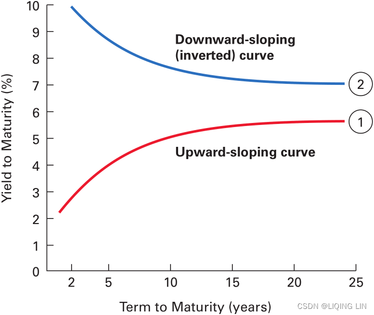
In certain economic conditions, the yield curve can be inverted. Long-term interest rates are lower than short-term interest rates. Such a condition occurs when the supply of money is tight. Investors are willing to forgo(/ fɔːrˈɡoʊ /放弃) long-term gains to preserve their wealth in the short-term. During periods of high inflation, where the inflation rate exceeds the rate of coupon interests, negative interest rates may be observed. Investors are willing to pay in the short-term just to secure their long-term wealth. The inverted yield curve is said to be downward sloping, as shown in the following graph:

Valuing a zero-coupon bond估值零利息债券

##################

Compound interest

Compound interest is interest calculated on the initial principal and also on the accumulated interest of previous periods of a deposit or loan. The effect of compound interest depends on frequency.

Assume an annual interest rate of 12%. If we start the year with $100 and compound only once, at the end of the year, the principal grows to $112 ( $\large P*(1+r*t) =100 * (1+0.12*1)$ = $112). Interest applied only to the principal is referred to as simple interest.

compounded monthly, n =12:

If we instead compound each month at 1%(monthly-compounded yield= $R=\frac{r}{n} = \frac{r}{frequency} = \frac{12%}{12}=1%$ ), we end up with more than $112 at the end of the year(T=1 year). That is, $\large FV= P * (1+\frac{r}{n})^{n*T} =PV * (1+R)^{t} =$ $\large 100 * (1+0.01)^{12}$ =112.68. (It's higher because we compounded more frequently.)

The future value (FV) of an investment of present value (PV or P) dollars earning interest at an annual rate of r compounded n times per year for a period of T years is $\large FV= P * (1+\frac{r}{n})^{n*T}$
P: the principal, the amount invested, or present value (PV)
r: the annual rate (in decimal form),
n: the number of times it is compounded or compound frequency.
$\large R=\frac{r}{n}$ is the interest per compounding period
T: the number of year
$\large t=n*T$ : is the number of compounding periods

If we known the monthly-compounded yield is 1%, and the value is $112.68 after one year, we want to calculate the present value: $\large pv=\frac{fv}{(1+\frac{r}{n})^{nT}}=\frac{fv}{(1+R)^{nT}}=\frac{112.68}{(1+0.01)^{1*12}}=100$

Continuously compounded returns compound the most frequently of all. Continuous compounding is the mathematical limit that compound interest can reach. It is an extreme case of compounding since most interest is compounded on a monthly, quarterly, or semiannual basis.

##################http://www.math.iupui.edu/~momran/m119/old/ch4h.htm

$\large BP = \sum_{T=1}^{nt}\frac{\frac{C}{n}}{(1+\frac{y}{n})^{T}} + \frac{FV}{(1+\frac{y}{n})^{nt}}$

C = the periodic coupon payment
or   is the coupon dollar amount paid at each time point T (T=1, 2, ..., nt)
if n = 1
0 ~ T1 ~ T2 ~ ... ~ t
| |
|   C | |
| ... C |
|   ...
| ...    C
y = the yield to maturity (YTM)
n: the number of times it is compounded
or the coupon payment frequency.
if n=1, then C = C : the coupon dollar amount paid at each time point T (T=1, 2, ..., t)
if n>1, then C = C/n : the coupon dollar amount paid at each time point T (T=1, 2, ..., nt)
$\large \frac{y}{n}$ : the yield per compounding period
T = the time period of payment (in years), T=1, 2, ..., t
t : the bond's maturity date
$\large n*t$ = the remaining number of periods from until the bond's maturity date t

A zero-coupon bond is a bond that does not pay any periodic interest(C=0) except on maturity(n=1), where the principal or face value is repaid. Zero-coupon bonds are also called pure discount bonds纯贴现债券.

A zero-coupon bond can be valued as follows:

Here, y is the annually-compounded yield年复合收益率 or rate of the bond, and t is the time remaining to the maturity of the bond. Let's take a look at an example of a five-year zero-coupon bond with a face value of $100. The yield is 5%, compounded annually. The price can be calculated as follows:

A simple Python zero-coupon bond calculator can be used to illustrate this example:

def zero_coupon_bond( par, y, t):
    """
    Price a zero coupon bond.
    
    :param par: face value of the bond.
    :param y: annual yield or rate of the bond.
    :param t: time to maturity, in years.
    """
    return par/(1+y)**t

Using the preceding example, we get the following result:

print( zero_coupon_bond(100, 0.05, 5) )

In the preceding example, we assumed that the investor is able to invest $78.35 at the prevailing(/ prɪˈveɪlɪŋ 现存的,现行) annual interest rate of 5% for 5 years, compounded annually.

Now that we have a zero-coupon bond calculator, we can use it to determine zero rates by bootstrapping引导 the yield curve, as explained in the next section.

#######################

effective interest rate

The effective interest rate is calculated as if compounded annually. The effective rate is calculated in the following way, where $\large r_{eff} = (1+\frac{r}{n})^{n} -1$ is the effective annual rate,

r the nominal rate, and
n the number of compounding periods per year (for example, 12 for monthly compounding):

For example, a nominal interest rate of 6% compounded monthly is equivalent to an effective interest rate of 6.17%.

$\large r_{eff} = (1+\frac{6%}{12})^{12} -1 \approx 1.0617-1 \approx 6.17%$

When the frequency of compounding is increased up to infinity (as for many processes in nature) the calculation simplifies to: $\LARGE r_{continuous} = e^{r_{eff}}-1$

If we increase the compound frequency to its limit, we are compounding continuously. While this may not be practical, the continuously compounded interest rate offers marvelously convenient properties. It turns out that the continuously compounded interest rate is given by:

$\LARGE r_{continuous}=ln(1+r_{eff})$ note: $\large r_{eff} = (1+\frac{r}{n})^{n} -1$

$\LARGE e^{r_c}=e^{r_{continuous}}=1+r_{eff} = (1+\frac{r}{n})^{n}$
$\large FV = PV * (1+R)^{nT} = p * (1+\frac{r}{n})^{nT}= p * (1+r_{eff})^{T} =p * e^{r_{c}*T}$

P: the principal, the amount invested, or present value (PV)
r: the annual rate (in decimal form),
T: the number of year
n: the number of times it is compounded or compound frequency in each T.
the interest rate is compounded n times per year
$\large R=\frac{r}{n}$ is the interest per compounding period
n*T: is the total number of compounding

When interest is compounded more frequently, the amount of interest earned in each increment of time becomes smaller, but the total amount of accumulated interest grows faster

What's so great about the continuously compounded rate (or return) that we will denote with $\LARGE r_{c}$ ? First, it's easy to scale it forward. Given a principal of (P), our final wealth over (T) years is given by:

$\LARGE w = A =FV= p * e^{r_{c}*T}$ If the interest is compounded continuously for T years at a rate of $\LARGE r_{c}$ per year, then the compounded amount is given by $\LARGE w = FV= p * e^{r_{c}*T}$

Note that e is the exponential function. For example, if we start with $100 and continuously compound at 8% over three years, the final wealth is given by:

$\LARGE w = A = p * e^{r_{c}*T}$ =

Discounting to the present value (PV or p) is merely compounding in reverse, so the present value of a future value (FV) compounded continuously at a rate of ( $\LARGE r_{c}$ ) is given by:

PV of FV received in (n) years $\LARGE PV=\frac{FV}{e^{r_{c}*T}}$

#######################Continuous Compound Interest

Spot and zero rates

As the compounding frequency increases (say, from compounded yearly to compounded daily), the future value of money reaches an exponential limit指数极限. That is to say, the value of $100 today will reach a future value of $100* $\LARGE e^{RT}$ when it is invested at a continuously compounded rate, R, for a period of time, T. If we discount these values for a security that pays $100 at a future time, T, with a continuously-compounded discount rate, R, its value at time 0 is $\LARGE e^{\frac{100}{RT}}$ . This rate is known as the spot rate即期利率.需要注意得是，即期利率不是一个能够直接观察到的市场变量，而是一个基于现金流折现法，通过对市场数据进行分析而得到的利率。

Spot rates represent the current interest rates for several maturities, should we want to borrow or lend money now. Zero rates( called zero-coupon interest rate or spot rate) represent the internal rate of return of zero-coupon bonds.

By deriving the spot rates of bonds with different maturities, we can construct the present yield curve through a bootstrapping引导 process using zero-coupon bonds.

Bootstrapping a yield curve引导收益率曲线

Short-term spot rates短期即期利率 can be derived directly from various short-term securities, such as zero-coupon bonds, T-bills国库券, notes, and eurodollar deposits欧洲美元存款. However, longer-term spot rates are typically derived from the prices of long-term bonds through a bootstrapping process, taking into account the spot rates of maturities that correspond to the coupon payment date. After obtaining short-term and long-term spot rates, the yield curve can then be constructed.

An example of bootstrapping the yield curve

Let's illustrate the bootstrapping of the yield curve with an example. The following table shows a list of bonds with different maturities and prices: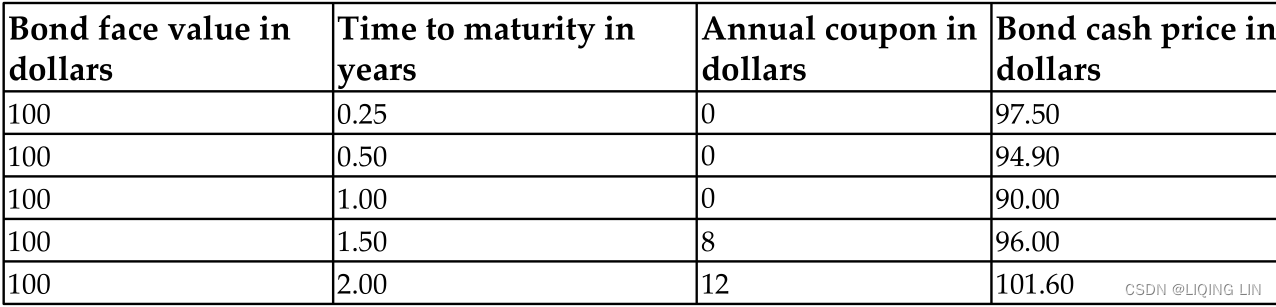

When T<=1 year, then C=0 Annual coupon (interest in dollars) payment

is replace with $\LARGE e^{R}$ , and N==T, and R is the sport rate

$\large \sum_{T=1}^{nt}\frac{\frac{C}{n}}{(1+\frac{y}{n})^{T}} + \frac{FV}{(1+\frac{y}{n})^{nt}}$ if n=1 ==> $\large \sum_{T=1}^{t}\frac{C}{(1+y)^{T}} + \frac{FV}{(1+y)^{t}}$ OR
==> $\LARGE BP = \sum_{t=1}^{T}\frac{C}{e^{Rt}} + \frac{PV_{T}}{e^{RT}}$

An investor in a three-month zero-coupon(interest payment C=0) bond today at $97.50 would earn interest of $2.50. The three-month spot rate can be calculated as follows:

Thus, the 3-month zero rate is 10.127% with continuous compounding. The spot rates of the zero-coupon bonds are shown in the following table:

import numpy as np

def spot_rate( price, T, par=100 ):
    return np.log(par/price)/T

print( "0.25 year's Sport rate:{:.5f}".format( spot_rate( 97.5, 0.25, par=100 ) ) )
print( "0.5 year's Sport rate(:{:.5f}".format( spot_rate( 94.9, 0.5, par=100 )  ) )
print( "1 year's Sport rate:{:.5f}".format( spot_rate( 90, 1., par=100 ) ) )

Using these spot rates, we can now price the 1.5-year bond (> 1year) as follows:

C = semi-annual coupon (interest) payment = 8/round(1.5) = 8/2 =4
==> $\LARGE BP = \sum_{t=1}^{T}\frac{C}{e^{Rt}} + \frac{PV_{T}}{e^{RT}}$

$\LARGE BP^{}=\frac{4}{e^{0.10469*0.5}} + \frac{4}{e^{0.10536*1.0}} + \frac{4}{e^{y*1.5}} + \frac{100}{e^{y*1.5}}$

The value of y (annual yield or rate of the bond) can easily be solved by rearranging the equation, as follows:

With the spot rate of the 1.5-year bond as 10.681%, we can use it to price the 2-year bond with coupons of $6 semi-annually, as follows:

C/2 = semiannual coupon payment = 12/2=6
$\LARGE BP = \sum_{t=1}^{T}\frac{C}{e^{Rt}} + \frac{PV_{T}}{e^{RT}}$

$\large BP^{}=\frac{6}{e^{0.10469*0.5}} + \frac{6}{e^{0.10536*1.0}} + \frac{6}{e^{0.106809*1.5}} + \frac{6}{e^{y*2}} + \frac{100}{e^{y*2}}$

Rearranging the equation and solving for y gives us the spot rate of the 2-year bond as 10.808.

Through this iterative procedure of calculating the spot rate of every bond in increasing order of maturity and using it in the next iteration, we obtain a list of spot rates of different maturities that we can use to construct the yield curve.

the yield curve bootstrapping class

The steps for writing the Python code to bootstrap the yield curve and running with a plot output are outlined as follows:

import math

class BootstrapYieldCurve( object ):
    def __init__(self):
        self.zero_rates = dict()  # self.zero_rates[T] = spot_rate
        self.instruments = dict() # self.instruments[T] = (par, coup, price, compounding_freq)
    ################## step 1 ##################   
    def add_instrument( self, par, T, coup, price, compounding_freq=2 ):
        # par : face value of the bond
        # price : current price of the bond
        # T as key : indexed by the maturity time T
        self.instruments[T] = (par, coup, price, compounding_freq)
        
    def get_maturities( self ):
        # return: a list of maturities Ts of added instruments in ascending order
        return sorted( self.instruments.keys() )
    
    # calculate the spot rate of a zero-coupon bond(interest payment=0) 
    # This method is called by bootstrap_zero_coupons()
    def zero_coupon_spot_rate(self, par, price, T):
        # return: the zero coupon spot rate with continuous compounding
        spot_rate = math.log( par/price ) / T
        return spot_rate
    
    ################## step 3 ################## 
    # calculate the annual yield rate of the bond when interest payment=0
    # OR
    # spot rates: zero-coupon interest rate or Zero rates
    # calculate the spot rates of the given zero-coupon bonds(interest payment=0)
    #   and adds them to the zero_rates dictionary, indexed by maturity.
    def bootstrap_zero_coupons( self ):
        # Bootstrap the yield curve with zero coupon(interest payment=0) instruments first.
        for (T, instrument ) in self.instruments.items():
            # self.instruments[T] = (par, coup, price, coumpounding_freq)
            par, coup, price, freq = instrument
            
            if coup==0:
                # the annual yield or rate of the bond when interest payment=0
                spot_rate = self.zero_coupon_spot_rate( par, price, T )
                self.zero_rates[T] = spot_rate
    
    # calculate the spot rate at a particular maturity period T
    def calculate_bond_spot_rate( self, T, instrument ):
        try:
            # par : face value of the bond
            par, coup, price, freq = instrument 
            periods = T*freq # 1.5 years * (1/0.5) = 1.5 * 2 = 3
                             #  2  years * (1.0.5) =    2 *2 = 4 
                                   #  8/2=4, 12/2=6 if freq=2   
            per_coupon = coup/freq # annual coupon payment/frequent
            value = price # current bond price
            
            for i in range( int(periods)-1 ):       # if freq=2
                t = (i+1)/float(freq) # 1/2 = 0.5, 2/2 = 1, 3/2 =1.5, ...
                
                # self.zero_rates[T] : def bootstrap_zero_coupons( self )
                spot_rate = self.zero_rates[t]
                
                # Coupon payment / e^( R*t ) 
                discounted_coupon = per_coupon * math.exp(-spot_rate*t)
                # value = current bond price
                value -= discounted_coupon
            
            # last_period == maturity T
            last_period = int(periods)/float(freq) # 3//2 = 1.5, 4//2=2.0
            spot_rate = -math.log( value/(par+per_coupon) )/last_period
            return spot_rate
        except:
            print("Error: spot rate not found for T=",t)
    
    ################## step 4 ################## 
    # calculate the annual yield rate of the bond when interest payment !=0
    # spot rates: zero-coupon interest rate or Zero rates
    # calculate the spot rates of non zero-coupon bonds(interest payment !=0) 
    # and adds them to the zero_rates dictionary, indexed by maturity T.
    def get_bond_spot_rates(self):
        """ 
        Get spot rates implied by bonds, using short-term instruments.
        # par : face value of the bond
        """
        for T in self.get_maturities(): # T_list in ascending order
            instrument = self.instruments[T]
            # self.instruments[T] = (par, coup, price, coumpounding_freq)
            par, coup, price, freq = instrument
            
            if coup !=0 :
                spot_rate = self.calculate_bond_spot_rate(T, instrument)
                self.zero_rates[T] = spot_rate
    
    ################## step 2 ################## 
    def get_zero_rates( self ):
        
        # calculate the annual yield rate of the bond when interest payment=0
        self.bootstrap_zero_coupons()
        
        # calculate the annual yield rate of the bond when interest payment!=0
        self.get_bond_spot_rates()
        
        # return a list of zero rates in ascending order of maturity..
        # self.get_maturities() : # T_list in ascending order
        return [ self.zero_rates[T] for T in self.get_maturities() ]

Instantiate the BootstrapYieldCurve class and add each bond's information from the preceding table:

yield_curve = BootstrapYieldCurve()
                        # (par, T, coup, price, compounding_freq=2 )
yield_curve.add_instrument(100, 0.25, 0., 97.5)
yield_curve.add_instrument(100, 0.5, 0., 94.9)
yield_curve.add_instrument(100, 1.0, 0., 90.)
yield_curve.add_instrument(100, 1.5, 8, 96., 2)
yield_curve.add_instrument(100, 2., 12, 101.6, 2)

ys = yield_curve.get_zero_rates()
ys

==> $\LARGE BP = \sum_{t=1}^{T}\frac{C}{e^{Rt}} + \frac{PV_{T}}{e^{RT}}$ ==>

$\LARGE BP^{}=\frac{4}{e^{0.10469*0.5}} + \frac{4}{e^{0.10536*1.0}} + \frac{4}{e^{y*1.5}} + \frac{100}{e^{y*1.5}}$ ==>
==>

xs = yield_curve.get_maturities()
xs

Calling the get_zero_rates() method in the class instance returns a list of spot rates in the same order as the maturities, which are stored in the x and y variables, respectively. Issue the following Python code to plot x and y on a graph:

%matplotlib inline
import matplotlib.pyplot as plt

fig = plt.figure( figsize=(12,8) )

plt.plot(xs,ys)
plt.title("Zero-Coupon Yield Curve(Zero Curve)", fontsize=14)
plt.ylabel( "Zero Rate (%)", fontsize=14 )
plt.xlabel( "Maturity in Years", fontsize=14 )
plt.show()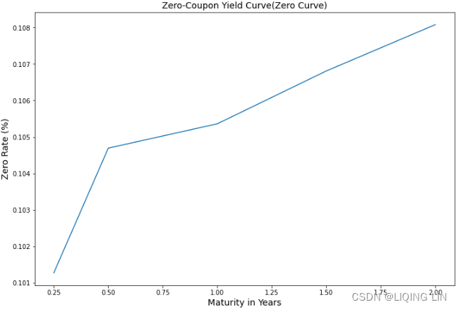

In a normal yield curve environment, where the interest rates increase as the maturities increase, we obtain an upward-sloping yield curve.

Forward rates远期利率

############################

The forward rate is the future yield on a bond. It is calculated using the yield curve.

We are trying to find the future interest rate $\large r_{1,2}$ for time period $\large (t_{1}, t_{2})$ , $\large t_{1}$ and $\large t_{2}$ expressed in years, given

the rate $\large r_{1}$ for time period $\large (0,t_{1})$
and rate $\large r_{2}$ for time period $\large (0,t_{2})$ .

To do this, we use the property that the proceeds from

investing at rate $\large r_{1}$ for time period $\large (0,t_{1})$
and then reinvesting those proceeds at rate $\large r_{1,2}$ for time period $\large (t_1,t_2)$
is equal to the proceeds from investing at rate $\large r_{2}$ for time period $\large (0,t_{2})$ .

$\large r_{1,2}$ depends on the rate calculation mode (simple, yearly compounded or continuously compounded), which yields three different results.

Simple rate

Yearly compounded rate

Continuously compounded rate

############################

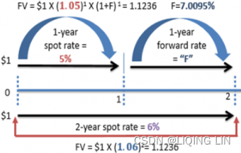
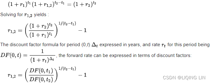
An investor who plans to invest at a later time may be curious to know what the future interest rate will look like, as implied by today's term structure of interest rates. For example, you might ask, What is the one-year spot rate one year from now? To answer this question, you can calculate forward rates for the period between T1 and T2 using this formula:

Here, $\LARGE r_{1}$ and $\LARGE r_{2}$ are the continuously-compounded annual interest rates at time periods $\LARGE T_{1}$ and $\LARGE T_{2}$ , respectively.

The following ForwardRates class helps us generate a list of forward rates from a list of spot rates:

# Continuously compounded rate
class ForwardRates( object ):
    
    def __init__(self):
        self.forward_rates = []
        self.spot_rates = dict()
        
    def add_spot_rate( self, T, spot_rate ):
        self.spot_rates[T] = spot_rate
        
    def calculate_forward_rate( self, T1, T2 ):
        # 0 ~ R1 ~ T1 ~ Forward rate ~ T2
        # |   --     R2       --        | 
        R1 = self.spot_rates[T1]
        R2 = self.spot_rates[T2]
        forward_rate = (R2*T2 - R1*T1)/(T2-T1)
        
        return forward_rate     
        
    def get_forward_rates( self ):
        """
        Returns a list of forward rates
        starting from the second time period.
        """
        periods = sorted( self.spot_rates.keys() )
        for T2, T1 in zip( periods, periods[1:] ):
            forward_rate = self.calculate_forward_rate(T1, T2)
            self.forward_rates.append( forward_rate )
            
        return self.forward_rates

Using spot rates derived from our preceding yield curve, we get the following result:

fr = ForwardRates()

fr.add_spot_rate( 0.25, 10.127 )
fr.add_spot_rate( 0.50, 10.469 )
fr.add_spot_rate( 1.00, 10.536 )
fr.add_spot_rate( 1.50, 10.681 )
fr.add_spot_rate( 2.00, 10.808 )

print( fr.get_forward_rates() )

Calling the get_forward_rates() method of the ForwardRates class returns a list of forward rates, starting from the next time period.

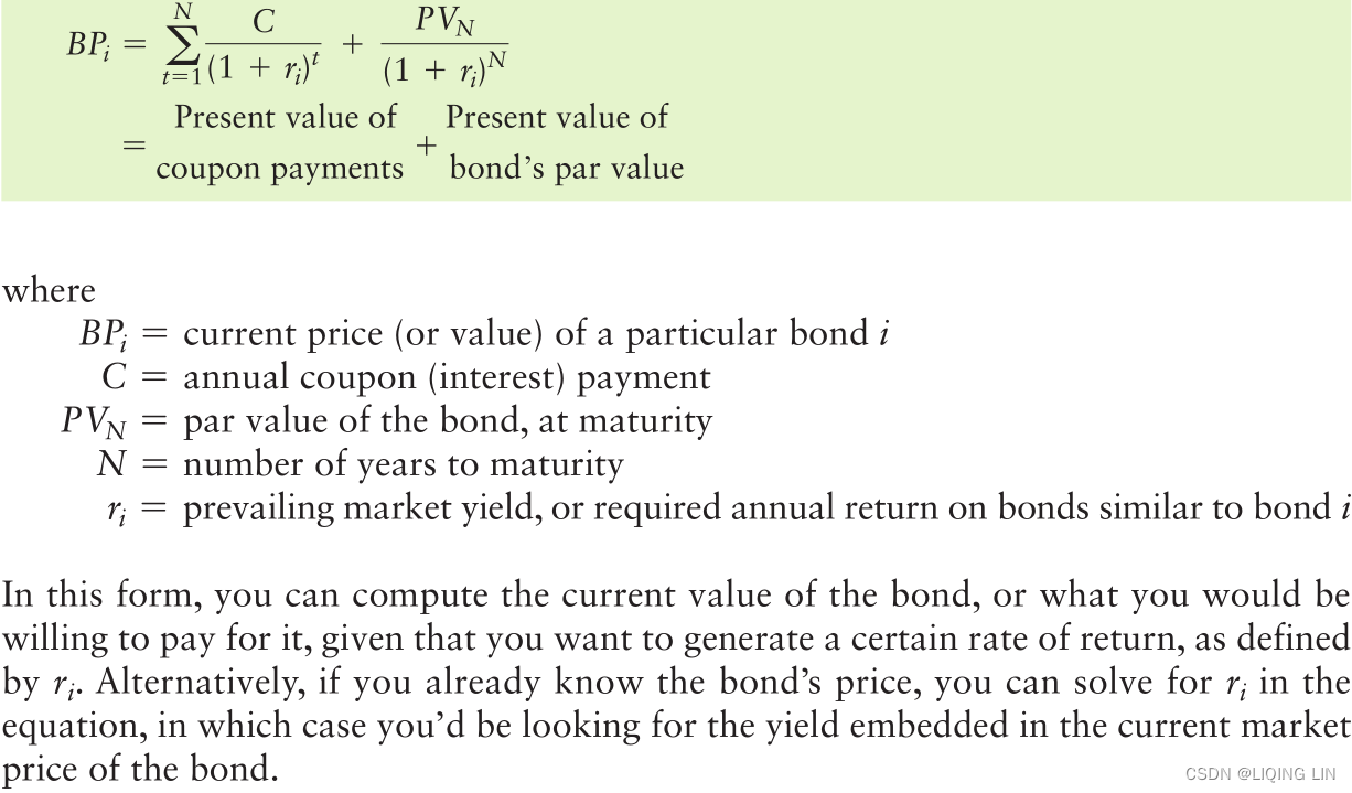
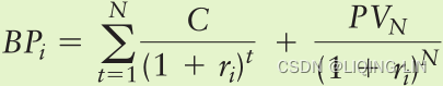
Calculating the yield to maturity

The yield to maturity (YTM到期收益率) measures the interest rate, as implied by the bond, which takes into account the present value of all the future coupon payments and the principal. It is assumed that bond holders can invest received coupons(or interest payments) at the YTM rate until the maturity of the bond; according to risk-neutral expectations, the payments received should be the same as the price paid for the bond.

$\large BP = \sum_{T=1}^{nt}\frac{\frac{C}{n}}{(1+\frac{y}{n})^{T}} + \frac{FV}{(1+\frac{y}{n})^{nt}}$

C = the periodic coupon payment
or   is the coupon dollar amount paid at each time point T (T=1, 2, ..., nt)
if n = 1
0 ~ T1 ~ T2 ~ ... ~ t
| |
|   C | |
| ... C |
|   ...
| ...    C
y = the yield to maturity (YTM)
n: the number of times it is compounded
or the coupon payment frequency.
if n=1, then C = C : the coupon dollar amount paid at each time point T (T=1, 2, ..., t)
if n>1, then C = C/n : the coupon dollar amount paid at each time point T (T=1, 2, ..., nt)
$\large \frac{y}{n}$ : the yield per compounding period
T = the time period of payment (in years), T=1, 2, ..., t
t : the bond's maturity date
$\large n*t$ = the remaining number of periods from until the bond's maturity date t

Let's take a look at an example of a 5.75% bond that will mature in 1.5 years(t=1.5) with a par value of 100(C=5.75%*100=5.75). The price of the bond is $95.0428 and coupons are paid semi-annually(n=2, c=C/n= 5.75/2=2.875). The pricing equation can be stated as follows:

$\large BP = \sum_{T=1}^{nt}\frac{\frac{C}{n}}{(1+\frac{y}{n})^{T}} + \frac{FV}{(1+\frac{y}{n})^{nt}} = \sum_{T=1}^{3=2*1.5}\frac{\frac{C}{n}}{(1+\frac{y}{n})^{T}} + \frac{100}{(1+\frac{y}{n})^{3}} = \sum_{T=1}^{2}\frac{\frac{C}{n}}{(1+\frac{y}{n})^{T}} + \frac{\frac{C}{n}+100}{(1+\frac{y}{n})^{3}} = \sum_{T=1}^{2}\frac{c}{(1+\frac{y}{n})^{T}} + \frac{c+100}{(1+\frac{y}{n})^{3}}$

To solve the YTM is typically a complex process, and most bond YTM calculators use Newton's method as an iterative process.
https://blog.csdn.net/Linli522362242/article/details/125662545
==>

The bond YTM calculator is illustrated by the following bond_ytm() function:

import scipy.optimize as optimize

def bond_ytm( price, par, T, coupon, freq=2, guess_y=0.05):
    freq = float( freq )
    periods = T*freq
    
    # dt = [ (i+1)/freq for T_i in range(int(periods)) ]
    dt = [ (i+1)/freq for i in range(int(periods))]
    # price : Bound_Price
    ytm_func = lambda y : sum([coupon/freq / (1+y/freq)**(freq*t_i)
                               for t_i in dt
                              ])+\
                          par / (1+y/freq)**(freq*T)\
                          - price
    # Bound_Price=ytm_func ==> ytm_func-Bound_Price=0
    return optimize.newton(ytm_func, guess_y)

Remember that we covered the use of Newton's method and other nonlinear function root solvers in https://blog.csdn.net/Linli522362242/article/details/125662545, Nonlinearity in Finance. For this YTM calculator function, we used the scipy.optimize package to solve the YTM.

Let's take a look at an example of a 5.75% bond(==> coupon=5.75% * par / nt) that will mature in 1.5 years with a par value of 100. The price of the bond is $95.0428 and coupons are paid semi-annually. The pricing equation can be stated as follows:

par = 100
T = 1.5             # deltaT = 1
freq_in_deltaT = 2  # dt = deltaT/freq_in_deltaT ==> dt = 0.5
coupon_at_Ti = 5.75 

bondPrice = 95.0428
ytm = bond_ytm(bondPrice,
               par, T, coupon_at_Ti, freq_in_deltaT)
print( "YTM: {}".format( ytm ) )

The YTM of the bond is 9.369%. Now we have a bond YTM calculator that can help us compare a bond's expected return with those of other securities.

$\large BP = \sum_{T=1}^{nt}\frac{\frac{C}{n}}{(1+\frac{y}{n})^{T}} + \frac{FV}{(1+\frac{y}{n})^{nt}}$ if n=1==>

The cash flows for the Ford bond consist of the purchase price for the bond today of $744.80, annual interest payments for Years 1 through 10 of $65, and a final interest payment of $65 plus the principal payment of $1,000, both at the end of Year 11.

par = 1000
T = 11             # deltaT = 1
freq_in_deltaT = 1  # dt = deltaT/freq_in_deltaT ==> dt = 1
coupon_at_Ti = 65 # Ti : 1,2,3...11=T

bondPrice = 744.80
ytm = bond_ytm(bondPrice,
               par, T, coupon_at_Ti, freq_in_deltaT)
print( "YTM: {:.2f}%".format( ytm*100 ) )

The yield to maturity on the bond is 10.52 percent, considerably higher than the coupon rate of interest of 6.5 percent($65/$1000) that the bond promises to pay. The fact that the yield to maturity is higher than the coupon rate is also consistent with the fact that the current market price of the bond is considerably less than the bond’s par value of $1,000. In fact, if the bond price were equal to the bond’s par value, then the yield to maturity and coupon rate of interest would be the same.

par = 1000
T = 11             # deltaT = 1
freq_in_deltaT = 1  # dt = deltaT/freq_in_deltaT ==> dt = 1
coupon_at_Ti = 65 # Ti : 1,2,3...11=T

bondPrice = 1000
ytm = bond_ytm(bondPrice,
               par, T, coupon_at_Ti, freq_in_deltaT)
print( "YTM: {:.2f}%".format( ytm*100 ) )

if the bond price were equal to the bond’s par value, then the yield to maturity and coupon rate of interest would be the same.

Calculating the price of a bond

When the YTM is known, we can get back the bond price in the same way we used the pricing equation. This is implemented by the bond_price() function:

def bond_price( par, T, ytm, coup, freq=2 ):
    freq = float(freq)
    periods = T*freq
    coupon = coup
    # dt = [ (i+1)/freq for T_i in range(int(periods)) ]
    dt = [ (i+1)/freq for i in range(int(periods))]
    # price : Bound_Price

    price = sum([coupon/freq / (1+ytm/freq)**(freq*t_i)
                 for t_i in dt
                ])+\
            par / (1+ytm/freq)**(freq*T)
    return price

Plugging in the same values from the earlier example, we get the following result:

par = 100
T = 1.5             # deltaT = 1
freq_in_deltaT = 2  # dt = deltaT/freq_in_deltaT ==> dt = 0.5
coupon_at_Ti = 5.75 # Ti

ytm_in_deltaT = 0.09369155345239522 
price = bond_price(par, T, 
                   ytm_in_deltaT, 
                   coupon_at_Ti, freq_in_deltaT)
print("Bond price:", price)

This gives us the same original bond price discussed in the earlier example, Calculating the yield to maturity. With the bond_ytm() and bond_price() functions, we can apply these for further uses in bond pricing, such as finding the bond's modified duration and convexity. These two characteristics of bonds are of importance to bond traders in helping them formulate制定 various trading strategies and hedge their risk.

Consider a $1,000 par value bond issued by AT&T (T) with a maturity date of 2032 and a stated coupon rate of 8.5 percent. On January 1, 2013, the bond had 20 years left to maturity, and the market’s required yield to maturity for similar rated debt was 7.5 percent. What is the value of the bond?

The cash flows for the AT&T bond consist of the value of the bond today, which we are trying to estimate, the annual interest payments for Years 1 through 20 of $85 each, and principal payment at the end of Year 20 equal to $1,085 (this is in addition to the $85 interest payment also at the end of Year 20).

par = 1000
T = 20             # deltaT = 1
freq_in_deltaT = 1 # dt = deltaT/freq_in_deltaT ==> dt = 1
coupon_at_Ti = 85 # Ti : 1,2,3...20=T

ytm_in_deltaT = 0.075
price = bond_price(par, T, 
                   ytm_in_deltaT, 
                   coupon_at_Ti, freq_in_deltaT)
print("Bond price:", price)

bondPrice = 1101.94
ytm = bond_ytm( bondPrice, 
                par, T, coupon_at_Ti, freq_in_deltaT)
print( "{:.2f}%".format( ytm*100 ) )

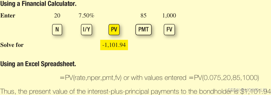
The value we calculated for the AT&T bond is $1,101.94, which exceeds the $1,000 par value of the bond. This reflects the fact that the market’s required yield to maturity on a comparable-risk bond is less than the coupon rate of interest paid on the bond of 8.5 percent($85/1000). In all likelihood, when the AT&T bonds were originally issued, they were issued at par because the market’s required yield to maturity on comparable-risk bonds was at or very near to the 8.5 percent coupon rate. Since the time of issue, however, market rates of interest have declined such that the bonds now sell at a premium(sell at >$1,000 par value). Thus if the bonds are sold for $1,101.94, they will yield a return of only 7.5 percent.

To illustrate this bond price formula in action, consider a 20-year, 9.5% bond priced to yield 10%. That is, the bond pays an annual coupon of 9.5% (or $95), has 20 years left to maturity, and should be priced to provide a market yield of 10%. We can now use Equation 11.3 to find the price of our bond.

par = 1000
T = 20             # deltaT = 1   
freq_in_deltaT = 1 # dt = deltaT/freq_in_deltaT ==> dt = 0.5
coupon_at_Ti = 95  # Ti : 1,2,3...20=T*1 if freq_in_deltaT =1
                   # Ti : 1,2,3...40=T*2 if freq_in_deltaT =2

ytm_in_deltaT = 0.1
price = bond_price(par, T, 
                   ytm_in_deltaT,
                   coupon_at_Ti, freq_in_deltaT)
print("Bond price:", price)

Note that because this is a coupon-bearing bond, we have an annuity of coupon payments of $95 a year for 20 years, plus a single cash flow of $1,000 that occurs at the end of year 20. Thus, we find the present value of the coupon annuity and then add that amount to the present value of the recovery of principal at maturity. In this particular case, you should be willing to pay about $958 for this bond, so long as you’re satisfied with earning 10% on your money.

Notice that this bond trades at a discount of $42.57 ($1,000 – $957.43). It trades at a discount because its coupon rate (9.5%) is below the market’s required return (10%). You can directly link the size of the discount on this bond to the present value of the difference between the coupons that it pays ($95) and the coupons that would be required if the bond matched the market’s 10% required return ($100). In other words, this bond’s coupon payment is $5 less than what the market requires, so if you take the present value of that difference over the bond’s life, you will calculate the size of the bond’s discount:

semiannual basis ==>

Reconsider the bond issued by AT&T (T) with a maturity date of 2032 and a stated coupon rate of 8.5 percent. AT&T pays interest to bondholders on a semiannual basis on January 15 and July 15. On January 1, 2013, the bond had 20 years left to maturity. The market’s required yield to maturity for a similarly rated debt was 7.5 percent per year or 3.75 percent(3.75%=7.5%/2.0) for six months. What is the value of the bond?

The cash flows for the AT&T bond consist of the value of the bond today, which we are trying to estimate, the semiannual interest payments for Periods 1 through 39 of $42.50 each($42.50=$85/2), and a final interest-plus-principal pay-ment at the end of Year 20 or Period 40 equal to $1,042.50.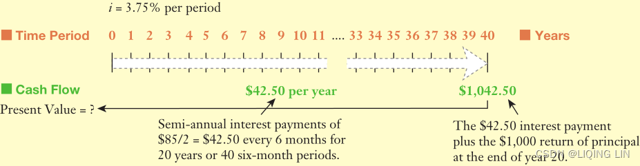

par = 1000
T = 20             # deltaT = 1   
freq_in_deltaT = 2 # dt = deltaT/freq_in_deltaT ==> dt = 0.5
coupon_at_Ti = 85  # Ti : 1,2,3...20=T*1 if freq_in_deltaT =1
                   # Ti : 1,2,3...40=T*2 if freq_in_deltaT =2

ytm_in_deltaT = 0.075
price = bond_price(par, T, 
                   ytm_in_deltaT,
                   coupon_at_Ti, freq_in_deltaT)
print("Bond price:", price)

bondPrice = 1102.75
ytm = bond_ytm(bondPrice,
               par, T, coupon_at_Ti, freq_in_deltaT)
print( "YTM: {:.2f}%".format( ytm*100 ) )
print( "YTM/{}: {:.2f}%".format( freq_in_deltaT, ytm*100/freq_in_deltaT ) )

Using semiannual compounding, we calculate a value of $1,102.75 for the AT&T bond compared to the $1,101.94 we calculated using annual compounding—this value is not vastly different没有太大的不同, but for a large investor buying thousands of bonds, this can certainly add up over time.

Bond duration

###################

Measuring Duration(Macaulay duration)

$\large BP = \sum_{T=1}^{nt}\frac{\frac{C}{n}}{(1+\frac{y}{n})^{T}} + \frac{FV}{(1+\frac{y}{n})^{nt}}$ ==>

Duration is a measure of the average maturity of a fixed-income security. The term average maturity may be confusing because bonds have only one final maturity date. An alternative definition of average maturity might be that it captures the average timing of the bond’s cash flow.

For a zero-coupon bond(C=0 and n=1) that makes only one cash payment on the final maturity date, the bond’s duration equals its maturity.
But because coupon-paying bonds make periodic interest payments, the average timing of these payments (i.e., the average maturity) is different from the actual maturity date(t). For instance, a 10-year bond that pays a 5% coupon each year(n=1, C = 5% * FV /n = 5%*FV) distributes a small cash flow in year 1, in year 2, and so on up until the last and largest cash flow in year 10.

Duration is a measure that puts some weight on these intermediate payments, so that the “average maturity” is a little less than 10 years.

Equation 11.8 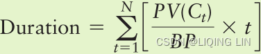Macaulay duration

where

$\large PV(C_t)$ = present value of a future coupon or principal payment
BP = current market price of the bond
t = year in which the cash flow (coupon or principal) payment is received
N = number of years to maturity

The duration measure obtained from Equation 11.8 is commonly referred to as Macaulay duration—named after the actuary who developed the concept.

Although duration is often computed using semiannual compounding, Equation 11.8 uses annual coupons and annual compounding to keep the ensuing discussion and calculations as simple as possible. Even so, the formula looks more formidable than it really is. If you follow the basic steps noted below, you’ll find that duration is not tough to calculate.

Step 1. Find the present value of each annual coupon or principal payment $\large [PV(C_t)]$ . Use the 现行prevailing YTM on the bond as the discount rate.
$\large PV(C_t)=\frac{C_t}{(1+YTM)^t}$ OR $\large PV(C_t)=\frac{C_t + FV}{(1+YTM)^t}$
Step 2. Divide this present value by the current market price of the bond (BP). This is the weight, or the fraction of the bond’s total value accounted for by each individual payment每笔单独付款占债券总价值的比例. $\large \frac{PV(C_t)}{BP}$
Because a bond’s value is just the sum of the present values of its cash payments, these weights must sum to 1.0.
Step 3. Multiply this weight by the year in which the cash flow is to be received (t). $\large \frac{PV(C_t)}{BP} \times t$
Step 4. Repeat steps 1 through 3 for each year in the life of the bond, and then add up the values computed in step 3.

Duration for a Single Bond

Table 11.1 (on page 435) illustrates the four-step procedure for calculating the duration of a 7.5%(n=1, C = 7.5% * FV /n = 7.5%*1000 = $75), 15-year bond priced at $957.20 to yield 8%.
Table 11.1 provides the basic input data:

Column (1) shows the year (t) in which each cash payment arrives.
Column (2) provides the dollar amount of each cash payment (coupons and principal) made by the bond.
Column (3) lists the present value of each cash flow, given an 8% discount rate (which is equal to the prevailing YTM on the bond).
- For example, in row 1 of Table 11.1, we see that in year 1 the bond makes a $75 coupon payment, and discounting that to the present at 8% reveals that the first coupon payment has a present value of $\large 69.44=PV(C_t)=\frac{C_t}{(1+YTM)^t} = \frac{75}{(1+0.08)^1}$ .
  $\large 64.30=PV(C_t)=\frac{C_t}{(1+YTM)^t} = \frac{75}{(1+0.08)^2}$
  $\large 338.88=PV(C_t)=\frac{C_t+FV}{(1+YTM)^t} = \frac{75+1000}{(1+0.08)^{15}}$
Next, in column 4 we divide the present value in column 3 by the current market price of the bond. If the present value of this bond’s first coupon payment is $69.44 and the total price of the bond is $957.20, then that first payment accounts for 7.25% of the bond’s total value (). Therefore, 7.25% is the “weight” given to the cash payment made in year 1.
is the “weight” given to the cash payment made in year 2

$\large \frac{PV(C_t)}{BP} = \frac{338.88}{957.20} = 0.3540$ is the “weight” given to the cash payment made in year 15
- If you sum the weights in column 4, you will see that they add to 1.0.
  Because a bond’s value is just the sum of the present values of its cash payments, these weights must sum to 1.0
Multiplying the weights from column 4 by the year (t) in which the cash flow arrives results in a time-weighted value for each of the annual cash flow streams shown in column 5.
$\large \frac{PV(C_t)}{BP} \times t= 0.0725 \times 1 = 0.0725$
$\large \frac{PV(C_t)}{BP} \times t= .0672 \times 2 = 0.1344$
$\large \frac{PV(C_t)}{BP} \times t= 0.3540 \times 15 = 5.3106$
Adding up all the values in column 5 yields the duration of the bond. As you can see, the duration of this bond is a lot less than its maturity(9.36 yr < 15 yr).

In addition, keep in mind that the duration on any bond will change over time as YTM and term to maturity change. For example, the duration on this 7.5%, 15-year bond will fall as the bond nears maturity and/or as the market yield (YTM) on the bond increases.

A bond’s price volatility is, in part, a function of its term to maturity and, in part, a function of its coupon. Unfortunately, there is no exact relationship between bond maturities and bond price volatilities with respect to interest rate changes. There is, however, a fairly close relationship between bond duration and price volatility—as long as the market doesn’t experience wide swings in interest rates. A bond’s duration can be used as a viable predictor of its price volatility only so long as the yield swings are relatively small (no more than 50 to 100 basis points, or so). That’s because as interest rates change, bond prices change in a nonlinear (convex) fashion. For example,

when interest rates fall, bond prices rise at an increasing rate.
When interest rates rise, bond prices fall at a decreasing rate.

The duration measure essentially predicts that as interest rates change, bond prices will move in the opposite direction in a linear fashion. This means that

when interest rates fall, bond prices will rise a bit faster than the duration measure would predict,
and when interest rates rise, bond prices will fall at a slightly slower rate than the duration measure would predict.

The bottom line最重要的是 is that the duration measure helps investors understand how bond prices will respond to changes in market rates, as long as those changes are not too large.

Modified Duration

The mathematical link between changes in interest rates and changes in bond prices involves the concept of modified duration. To find modified duration, we simply take the (Macaulay) duration for a bond (as found from Equation 11.8and $\large PV(C_t)=\frac{C_t+FV || C_t}{(1+YTM)^t}$ ) and adjust it for the bond’s yield to maturity.

Equation 11.9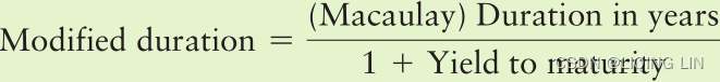

Thus, the modified duration for the 15-year bond discussed above is Note that here we use the bond’s computed (Macaulay) duration of 9.36 years and the same YTM we used to compute duration in Equation 11.8; in this case, the bond was priced to yield 8%, so we use a yield to maturity of 8%.

To determine, in percentage terms, how much the price of this bond would change as market interest rates increased by 50 basis points from 8% to 8.5%,
we multiply the modified duration value calculated above first by –1 (because of the inverse relationship between bond prices and interest rates) and then by the change in market interest rates. That is,

Thus, a 50-basis-point (or 0.5% = ½ of 1%) increase in market interest rates will lead to an approximate 4.33% drop in the price of this 15-year bond. Such information is useful to bond investors seeking—or trying to avoid—price volatility.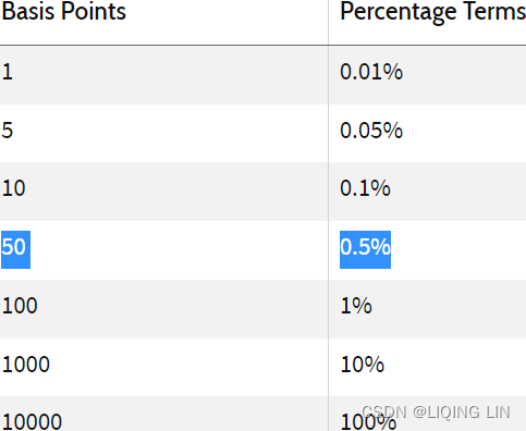

Effective Duration

One problem with the duration measures that we’ve studied so far is that they do not always work well for bonds with embedded options such as callable bonds. That is, the duration measures we’ve been using assume that the bond’s future cash flows ( $\large C_t+FV$ or $\large C_t$ ) are paid as originally scheduled through maturity, but that may not be the case with callable bonds (or convertible bonds or bonds with other types of options attached to them). An alternative duration measure that is used for these types of bonds is the effective duration. To calculate effective duration (ED), you use Equation 11.11:

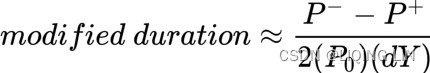
= the new price of the bond if market interest rates $\large r_i$ go down
the price of the bond from a decrease in yield by dY
= the new price of the bond if market interest rates $\large r_i$ go up
the price of the bond from an increase in yield by dY
$\large BP$ = the original price of the bond
$\large \Delta r_i$ = the change in market interest rates
dY is the given change in yield

Suppose you want to know the effective duration of a 25-year bond that pays a 6% coupon semiannually(2). The bond is currently priced at $882.72 for a yield of 7%.

par = 1000
T = 25             # deltaT = 1   
freq_in_deltaT = 2 # dt = deltaT/freq_in_deltaT ==> dt = 0.5
coupon_at_Ti = 60  # Ti : 1,2,3...20=T*1 if freq_in_deltaT =1
                   # Ti : 1,2,3...40=T*2 if freq_in_deltaT =2

ytm_in_deltaT = 0.07
price = bond_price(par, T, 
                   ytm_in_deltaT,
                   coupon_at_Ti, freq_in_deltaT)
print("Bond price:", price)

$\large BP$

Now suppose the bond’s yield goes up by 0.5%
( use 50-basis-point = 50% * 1% = 0.5% change in yield )
change in yield) to 7.5%. At that yield the new price would be $831.74 (using a calculator, N = 50 = 25*2, I = 3.75 = 7%/2, PMT = 30 = 6%/2 * 1000, and PV = 1,000).

par = 1000
T = 25             # deltaT = 1   
freq_in_deltaT = 2 # dt = deltaT/freq_in_deltaT ==> dt = 0.5
coupon_at_Ti = 60  # Ti : 1,2,3...20=T*1 if freq_in_deltaT =1
                   # Ti : 1,2,3...40=T*2 if freq_in_deltaT =2

ytm_in_deltaT = 0.075
price = bond_price(par, T, 
                   ytm_in_deltaT,
                   coupon_at_Ti, freq_in_deltaT)
print("Bond price:", price)

What if the yield drops by 0.5%
( use 50-basis-point = 50% * 1% = 0.5% change in yield )
to 6.5%? In that case, the price rises to $938.62 (N = 50, I = 3.25, PMT = 30, PV = 1,000).

par = 1000
T = 25             # deltaT = 1   
freq_in_deltaT = 2 # dt = deltaT/freq_in_deltaT ==> dt = 0.5
coupon_at_Ti = 60  # Ti : 1,2,3...20=T*1 if freq_in_deltaT =1
                   # Ti : 1,2,3...40=T*2 if freq_in_deltaT =2

ytm_in_deltaT = 0.065
price = bond_price(par, T, 
                   ytm_in_deltaT,
                   coupon_at_Ti, freq_in_deltaT)
print("Bond price:", price)

Now we can use Equation 11.11 to calculate the bond’s effective duration.

Effective duration = $\large \frac{938.62 - 831.74}{2 \times 882.72 \times 0.005} = 12.11$

This means that if interest rates rise or fall by a full percentage point一个百分点(50-basis-point = 50% * 1% = 0.5% change in yield, 0.5%*2=1%), the price of the bond would fall or rise by approximately 12.11%.
Note that you can use effective duration in place of modified duration in Equation 11.10to find the percent change in the price of a bond when interest rates move by more or less than 1.0%.

When calculating the effective duration of a callable bond, one modification may be necessary.

If the calculated price of the bond when interest rates fall is greater than the bond’s call price, then use the call price in the equation rather than and proceed as before.

###################

Duration is a sensitivity measure of bond prices to yield changes. Some duration measures are

effective duration,
Macaulay duration,
and modified duration.

The type of duration that we will discuss is modified duration, which measures the percentage change in bond price with respect to a percentage change in yield衡量债券价格的百分比变化相对于收益率百分比变化 (typically 1% or 100 basis points (bps)).

The higher the duration of a bond, the more sensitive it is to yield changes.
Conversely, the lower the duration of a bond, the less sensitive it is to yield changes.

The modified duration of a bond can be thought of as the first derivative of the relationship between price and yield:
VS
Here:

dY is the given change in yield
$\large P^{-}$ is the price of the bond from a decrease in yield by dY
$\large P^{+}$ is the price of the bond from an increase in yield by dY
$\large P_{0}$ is the initial price of the bond

It should be noted that the duration describes the linear price-yield relationship for a small change in Y. Because the yield curve is not linear, using a large value of dY does not approximate the duration measure well.

The implementation of the modified duration(should be called Effective duration) calculator is given in the following bond_mod_duration() function.

It uses the bond_ytm() function as discussed earlier in this chapter, Calculating the yield to maturity, to determine the yield of the bond with the given initial value.
Also, it uses the bond_price() function to determine the price of the bond with the given change in yield:

def bond_mod_duration( price, par, T, coup, freq, dy=0.01 ):
    # dy : the change in market interest rates
    # 0.01 : 1-basis-point change in yield
    ytm = bond_ytm( price, par, T, coup, freq )
    
    ytm_minus = ytm - dy
    price_minus = bond_price( par, T, ytm_minus, coup, freq )
    # the price of the bond from a decrease in yield by dY
    # or the new price of the bond if market interest rate(ytm) go down
    print( 'the price of the bond from a decrease in yield by {}: {:.4f}'.format(dy, price_minus) )
    
    ytm_plus = ytm + dy
    price_plus = bond_price( par, T, ytm_plus, coup, freq )
    # the price of the bond from an increase in yield by dY
    # the new price of the bond if market interest rate(ytm) go up
    print( 'the price of the bond from an increase in yield by {}: {:.4f}'.format(dy, price_plus) )
    
    mduration = ( price_minus-price_plus )/( 2*price*dy )
    
    return mduration

We can find out the modified duration of the 5.75% bond(coupon payment: 5.75%*100=$5.75) discussed earlier, in Calculating the yield to maturity, which will mature in 1.5 years(t) with a par value of 100 and a bond price of 95.0428(BP):
$\large BP = \sum_{T=1}^{nt}\frac{\frac{C}{n}}{(1+\frac{y}{n})^{T}} + \frac{FV}{(1+\frac{y}{n})^{nt}}$ n=2 since this bond will pay a fixed amount of interest semi-annually,
vs

mod_duration = bond_mod_duration( 95.0428, 100, 1.5, 5.75, 2 )
print( mod_duration )

The modified duration of the bond is 1.392 years(< the maturity of bond 1.5 yr). Duration is a measure of the average maturity of a fixed-income security. The term average maturity may be confusing because bonds have only one final maturity date. An alternative definition of average maturity might be that it captures the average timing of the bond’s cash flow.

Suppose you want to know the effective duration of a 25-year bond that pays a 6% coupon semiannually(n=2). The bond is currently priced at $882.72 for a yield of 7%.
Now suppose the bond’s yield goes up by 0.5%
( use 50-basis-point = 50% * 1% = 0.5% change in yield ) change in yield )
to 7.5%. At that yield the new price would be $831.74 (using a calculator, N = 50 = 25*2, I = 3.75 = 7%/2, PMT = 30 = 6%/2 * 1000, and PV = 1,000).
What if the yield drops by 0.5% to 6.5%? In that case, the price rises to $938.62 (N = 50, I = 3.25, PMT = 30, PV = 1,000). $\large BP = \sum_{T=1}^{nt}\frac{\frac{C}{n}}{(1+\frac{y}{n})^{T}} + \frac{FV}{(1+\frac{y}{n})^{nt}}$

par = 1000
T = 25             # deltaT = 1   
freq_in_deltaT = 2 # dt = deltaT/freq_in_deltaT ==> dt = 0.5
coupon_at_Ti = 60  # Ti : 1,2,3...20=T*1 if freq_in_deltaT =1
                   # Ti : 1,2,3...40=T*2 if freq_in_deltaT =2

ytm_in_deltaT = 0.07

bondPrice = 882.72

dy=0.005 # use 50-basis-point = 50% * 1% = 0.5% change in yield
mod_duration = bond_mod_duration( bondPrice, par, T, coupon_at_Ti, freq_in_deltaT, dy)
print( mod_duration )

Bond convexity

Convexity is the sensitivity measure of the duration of a bond to yield changes衡量债券久期对收益率变化的敏感度. Think of convexity as the second derivative of the relationship between the price and yield: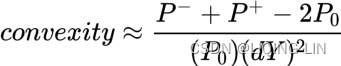

Bond traders use convexity as a risk-management tool to measure the amount of market risk in their portfolio衡量其投资组合中的市场风险量.

Higher-convexity portfolios are less affected by interest-rate volatilities than lower-convexity portfolios, given the same bond duration and yield.
As such, higher-convexity bonds are more expensive than lower-convexity ones, everything else being equal.

The implementation of a bond convexity is given as follows:

def bond_convexity( price, par, T, coup, freq, dy=0.01 ):
    # dy : the change in market interest rates
    # 0.01 : 1-basis-point change in yield    
    ytm = bond_ytm( price, par, T, coup, freq )
    
    ytm_minus = ytm-dy
    price_minus = bond_price( par, T, ytm_minus, coup, freq )
    # the price of the bond from a decrease in yield by dY
    # or the new price of the bond if market interest rate(ytm) go down
    print( 'the price of the bond from a decrease in yield by {}: {:.4f}'.format(dy, price_minus) )
    
    ytm_plus = ytm + dy
    price_plus = bond_price(par, T, ytm_plus, coup, freq)
    # the price of the bond from an increase in yield by dY
    # the new price of the bond if market interest rate(ytm) go up
    print( 'the price of the bond from an increase in yield by {}: {:.4f}'.format(dy, price_plus) )
    
    convexity = (price_minus + price_plus - 2*price)/(price*dy**2)
    
    return convexity

We can now find the convexity of the 5.75% bond discussed earlier, in Calculating the yield to maturity section, which will mature in 1.5 years with a par value of 100 and a bond price of 95.0428:

convexity = bond_convexity( 95.0428, 100, 1.5, 5.75, 2 )
print( convexity )

The convexity of the bond is 2.63. For two bonds with the same par value( $\large FV$ ), coupon $\large \frac{C}{n}$ , and maturity( $\large t$ ), their convexity may be different, depending on their location on the yield curve. $\large BP = \sum_{T=1}^{nt}\frac{\frac{C}{n}}{(1+\frac{y}{n})^{T}} + \frac{FV}{(1+\frac{y}{n})^{nt}}$ Higher-convexity bonds will exhibit higher price changes for the same change in yield(dY).

Short–rate modeling

In short-rate modeling, the short-rate, r(t), is the spot rate即期利率 at a particular time. It is described as a continuously-compounded连续复利, annualized interest rate term for an infinitesimally short period of time on the yield curve. The short-rate takes on the form of a stochastic variable in interest-rate models, where the interest rates may change by small amounts at every point in time. Short-rate models attempt to model the evolution of interest rates over time, and hopefully describe the economic conditions at certain periods.

Short-rate models are frequently used in the evaluation of interest-rate derivatives利率衍生品的评估. Bonds, credit instruments, mortgages, and loan products are sensitive to interest-rate changes. Short-rate models are used as interest rate components in conjunction with pricing implementations, such as numerical methods, to help price such derivatives.

Interest-rate modeling is considered a fairly complex topic since interest rates are affected by a multitude of factors, such as

economic states经济状况,
political decisions政策决定,
government intervention政府干预,
and laws of supply and demand供求规律 .

A number of interest-rate models have been proposed to account for various characteristics of interest rates.

In this section, we will take a look at some of the most popular one-factor short-rate models单因素短期利率模型 used in financial studies, namely,

the Vasicek,
Cox-Ingersoll-Ross,
Rendleman and Bartter,
and Brennan and Schwartz models.

Using Python, we will perform a one-path simulation to obtain a general overview of the interest-rate path process. Other models commonly discussed in finance include the Ho-Lee, Hull-White, and Black-Karasinki.

#########################

mpf4_定价欧式美式障碍Options_CRR_Leisen-Reimer_Greeks_二叉树三叉树网格_Finite differences(显式隐式)Crank-Nicolson_Imp波动率_LIQING LIN的博客-CSDN博客

Brownian motion(Wiener process维纳过程)

以W(t）表示运动中一微粒从时刻t=0到时刻t>0的位移的横坐标（同样也可以讨论纵坐标），且设 $\large W_0$ =0，根据爱因斯坦1905年提出的理论，微粒的这种运动是由于受到大量随机的相互独立的分子的碰撞的结果. 于是，粒子在时段（s,t]上的位移可以看作是许多微小位移的代数和. 则 $\large W_t - W_s$ 服从正态分布。

The Wiener process $\large W_t$ is characterised by the following properties:

$\large W_0$ =0 OR
W has independent increments:
for every t>0, the future increments $\large W_{t+u} - W_t$ , u>=0, are independent of the past values $\large W_s$ , s<=t,
s <= t <= t+u
W has Gaussian increments: $\large W_{t+u} - W_t$ is normally distributed with mean 0 and variance u, $\large W_{t+u} - W_t \sim ~ N(0,u)$
W has continuous paths: is continuous in t

That the process has independent increments means that if then $\large W_{t1} - W_{s1}$ and $\large W_{t2} - W_{s2}$ are independent random variables, and the similar condition holds for n increments.

Basic properties of a one-dimensional Wiener process

The unconditional probability density function follows a normal distribution with mean = 0 and variance = t, at a fixed time t: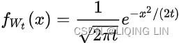

normal distribution:

The expectation is zero:

The variance, using the computational formula, is t:

These results follow immediately from the definition that increments have a normal distribution, centered at zero. Thus

######################

The Vasicek model

In finance, the Vasicek model is a mathematical model describing the evolution of interest rates. It is a type of one-factor short-rate model as it describes interest rate movements as driven by only one source of market risk. The model can be used in the valuation估值 of interest rate derivatives, and has also been adapted for credit markets. It was introduced in 1977 by Oldřich Vašíček,[1] and can be also seen as a stochastic investment model.

In the one-factor Vasicek model, the short-rate is modeled as a single stochastic factor单个随机因素:

$\large r(t)$ Process level at date t

The drift coefficient $\LARGE K * (\theta - r_t)$ depends on the current value of $\large r(t)$ .
If $\large r(t)$ is less than $\large \theta$ , then the drift coefficient is positive;
if $\large r(t)$ is greater than $\large \theta$ , then it is negative. Thus, the interest-rate tends to revert to its reversion level $\large \theta$ at a rate which depends upon the speed of adjustment K
$\large \theta$ Long-term mean of the process
All future trajectories of $\large r(t)$ will evolve around a mean level $\large \theta$ in the long run;
K Mean-reversion factor
"speed of reversion回归速度". K characterizes the velocity at which such trajectories will regroup around $\large \theta$ in time; K 表征这些轨迹将在时间 $\large \theta$ 周围重新组合的速度
$\large W_t$ is a Wiener process(Standard Brownian motion) under the risk neutral framework modelling the random market risk factor, in that it models the continuous inflow of randomness into the systemhttps://blog.csdn.net/Linli522362242/article/details/125355166
The standard deviation parameter, $\large \sigma$ , determines the volatility of the interest rate and in a way characterizes the amplitude/ˈæmplɪtuːd/ of the instantaneous randomness inflow.
$\large \sigma$ Constant volatility parameter （The spread(range) of the value of $\large r(t)$ ）

$\large \sigma$ :"instantaneous volatility瞬时波动率", measures instant by instant the amplitude of randomness entering the system. Higher $\large \sigma$ implies more randomness

$\large \frac{\sigma^2}{2K}$ : "long term variance". All future trajectories of r will regroup around the long term mean with such variance after a long time.
K and $\large \sigma$ tend to oppose each other:
increasing $\large \sigma$ increases the amount of randomness entering the system, but at the same time increasing K amounts to increasing the speed at which the system will stabilize statistically around the long term mean $\large \theta$ with a corridor(狭长地带,走廊) of variance(OR $\large \sigma^2$ ) determined also by K. This is clear when looking at the long term variance,
increases $\large \frac{\sigma^2}{2K}$ by increasing $\large \sigma$ but decreases $\large \frac{\sigma^2}{2K}$ by increasing K.

Here, K, θ, and σ are constants, and σ is the instantaneous/ˌɪnstənˈteɪniəs/ standard deviation. W(t) is the random Wiener process. The Vasicek follows an Ornstein–Uhlenbeck stochastic process, where the model reverts around the mean, θ, with K, the speed of mean reversion. As a result, the interest rates( $\large r_t$ ) may become negative, which is an undesirable不受欢迎的 property in most normal economic conditions.
(Making the long term mean $\large \theta$ stochastic to another SDE is a simplified version of the cointelation SDEhttps://blog.csdn.net/Linli522362242/article/details/96593981)
https://blog.csdn.net/Linli522362242/article/details/125355166
since and are identical in distribution, where Z is a standard normal variable.(==
)

$\large dr_t = K*(\theta - r_t) *dt + \sigma* \sqrt{dt}* dZ_t$

$\large r_{t+\Delta t} = r_t + dr_t$

To help us understand this model, the following code generates a list of interest rates:

import math
import numpy as np

def vasicek( r0, K, theta, sigma, T=1., N=10, seed=777 ):
    # r0 : the initial rate of interest at t=0
    # K : "speed of Mean-reversion
    # theta : All future trajectories of r(t) will evolve around a 'mean' level 'theta' in the long run
    # sigma : determines the volatility of the interest rate and amplitude(range of r(t)) 
    # T : the period in terms of number of years
    # N : the number of intervals for the modeling process
    # W : a Wiener process(Standard Brownian motion)
    #     modelling the random market risk factor(under the risk neutral framework)
    np.random.seed( seed )
    
    dt = T/float(N)
    rates = [r0]
                                                 # Z is a standard normal variable
    for i in range(N):                           # dW = sqrt(dt) * dZ
        dr = K * (theta - rates[-1]) * dt + sigma* math.sqrt(dt) * np.random.normal()
        rates.append( rates[-1]+dr )
    # returns a list of time periods and interest rates
    return range(N+1), rates

The vasicek() function returns a list of time periods and interest rates from the Vasicek model. It takes in a number of input arguments: r0 is the initial rate of interest at t=0; K , theta , and sigma are constants; T is the period in terms of number of years; N is the number of intervals for the modeling process; and seed is the initialization value for NumPy's standard normal random-number generator.

Assume that the current interest rate is close to zero at 0.5%, the long term mean level theta is 0.15, and the instantaneous volatility sigma is 5%. We will use a T value of 10 and an N value of 200 to model the interest rates for different speeds of mean reversion, K, with values of 0.002, 0.02, and 0.2 :

%matplotlib inline
import matplotlib.pyplot as plt

fig = plt.figure( figsize=(12,8) )

# r0 : the initial rate of interest at t=0
r0 = 0.005
# K : "speed of Mean-reversion
# theta : All future trajectories of r(t) will evolve around a 'mean' level 'theta' in the long run
theta = 0.15
# sigma : determines the volatility of the interest rate and amplitude(range of r(t)) 
sigma = 0.05
# T : the period in terms of number of years
T = 10
# N : the number of intervals for the modeling process
N = 200    
# K : "speed of Mean-reversion

K_list = [0.002, 0.02, 0.2]
colors = ['k','g','b']

for index, K in enumerate(K_list):
    N_plus_1, rate_list = vasicek( r0, K, theta ,sigma, T, N )
    plt.plot( N_plus_1, rate_list,
              label='K=%s' % K,
              c = colors[index]
            )
    
plt.axhline(y=theta, ls='--', c='r') # Long-term mean(theta) of the process
plt.annotate( r'Long-term mean(${\theta}$)',

              ha='right',

              va='top',

              xytext=(80, theta - 0.01), #The xytext parameter specifies the text position               

              xy=(80, theta),     #The xy parameter specifies the arrow's destination 

              arrowprops=dict(facecolor='blue', headwidth=10, headlength=4, width=2 ),

              #arrowprops={'facecolor':'blue', 'headwidth':10, 'headlength':4, 'width':2} #OR
              fontsize=14
            )

plt.legend( loc='upper left' , fontsize=14)
plt.ylabel('The interest rate', fontsize=14)
plt.xlabel('The time t', fontsize=14)
plt.title('Vasicek model', fontsize=14)
plt.show()

After running the preceding commands, we get the following graph:
In this example, we are running just one simulation to see what the interest rates from the Vasicek model looks like. Observe that interest rates did become negative at some point. With higher levels of speed for mean reversion, K , the process reaches its long-term level of 0.15(the model reverts around the mean, θ=0.15) sooner.

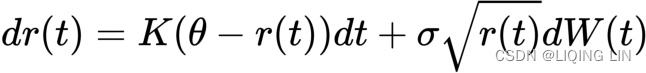
The Cox-Ingersoll-Ross model

The Cox-Ingersoll-Ross (CIR) model is a one-factor model that was proposed to address the negative interest rates found in the Vasicek model.(It is a type of one-factor short-rate model as it describes interest rate movements as driven by only one source of market risk)==> $\LARGE dr_t = K*(\theta - r_t) *dt + \sigma* \sqrt{dt}* dZ_t$ . The process is given as follows:
==> $\LARGE dr_t = K * (\theta - r_t) * dt + \sigma * \sqrt{r_t}* \sqrt{dt} * dZ_t$
$\LARGE r_{t+\Delta t} = r_t + dr_t$

$\large r(t)$ Process level at date t

The drift coefficient $\LARGE K * (\theta - r_t)$ depends on the current value of $\large r(t)$ .
If $\large r(t)$ is less than $\large \theta$ , then the drift coefficient is positive;
if $\large r(t)$ is greater than $\large \theta$ , then it is negative. Thus, the interest-rate tends to revert to its reversion level $\large \theta$ at a rate which depends upon the speed of adjustment K
$\large \theta$ Long-term mean of the process
All future trajectories of $\large r(t)$ will evolve around a mean level $\large \theta$ in the long run;
K Mean-reversion factor
"speed of reversion回归速度". K characterizes the velocity at which such trajectories will regroup around $\large \theta$ in time; K 表征这些轨迹将在时间 $\large \theta$ 周围重新组合的速度
$\large W_t$ is a Wiener process(Standard Brownian motion) under the risk neutral framework modelling the random market risk factor, in that it models the continuous inflow of randomness into the systemhttps://blog.csdn.net/Linli522362242/article/details/125355166
The standard deviation parameter, $\large \sigma$ , determines the volatility of the interest rate and in a way characterizes the amplitude/ˈæmplɪtuːd/ of the instantaneous randomness inflow.
$\large \sigma$ Constant volatility parameter （The spread(range) of the value of $\large r(t)$ ）

$\large \sigma$ :"instantaneous volatility瞬时波动率", measures instant by instant the amplitude of randomness entering the system. Higher $\large \sigma$ implies more randomness

$\large \frac{\sigma^2}{2K}$ : "long term variance". All future trajectories of r will regroup around the long term mean with such variance after a long time.
K and $\large \sigma$ tend to oppose each other:
increasing $\large \sigma$ increases the amount of randomness entering the system, but at the same time increasing K amounts to increasing the speed at which the system will stabilize statistically around the long term mean $\large \theta$ with a corridor(狭长地带,走廊) of variance(OR $\large \sigma^2$ ) determined also by K. This is clear when looking at the long term variance,
increases $\large \frac{\sigma^2}{2K}$ by increasing $\large \sigma$ but decreases $\large \frac{\sigma^2}{2K}$ by increasing K.

The term $\large \sqrt{r(t)}$ increases the standard deviation as the short-rate increases. Now the vasicek() function can be rewritten as the CIR model in Python:

import math
import numpy as np

def CIR( r0, K, theta, sigma, T=1, N=10, seed=777 ):
        # r0 : the initial rate of interest at t=0
    # K : "speed of Mean-reversion
    # theta : All future trajectories of r(t) will evolve around a 'mean' level 'theta' in the long run
    # sigma : determines the volatility of the interest rate and amplitude(range of r(t)) 
    # T : the period in terms of number of years
    # N : the number of intervals for the modeling process
    # W : a Wiener process(Standard Brownian motion)
    #     modelling the random market risk factor(under the risk neutral framework)
    np.random.seed(seed)
    
    dt = T/float(N)
    rates = [r0]
                                               # dW = sqrt(dt) * dZ  
    for i in range(N):                         # Z is a standard normal variable
        dr = K * ( theta-rates[-1] ) * dt +\
                sigma * math.sqrt( rates[-1] ) * math.sqrt(dt)*np.random.normal()
        rates.append( rates[-1] + dr )
        
    # returns a list of time periods and interest rates
    return range(N+1), rates

Using the same example given in the The Vasicek model section, assume that the current interest rate is 0.5%, theta is 0.15 , and sigma is 0.05 . We will use a T value of 10 and N of 200 to model the interest rates with different speeds of mean reversion, K , using values of 0.002 , 0.02 , and 0.2:

%matplotlib inline
import matplotlib.pyplot as plt

fig = plt.figure( figsize=(12,8) )

# r0 : the initial rate of interest at t=0
r0 = 0.005
# K : "speed of Mean-reversion
# theta : All future trajectories of r(t) will evolve around a 'mean' level 'theta' in the long run
theta = 0.15
# sigma : determines the volatility of the interest rate and amplitude(range of r(t)) 
sigma = 0.05
# T : the period in terms of number of years
T = 10
# N : the number of intervals for the modeling process
N = 200    
# K : "speed of Mean-reversion

K_list = [0.002, 0.02, 0.2]
colors = ['k','g','b']

for index, K in enumerate(K_list):
    N_plus_1, rate_list = CIR( r0, K, theta ,sigma, T, N )
    plt.plot( N_plus_1, rate_list,
              label='K=%s' % K,
              c = colors[index]
            )

plt.axhline(y=theta, ls='--', c='r') # Long-term mean(theta) of the process

plt.annotate( r'Long-term mean(${\theta}$)',

              ha='left',

              va='top',

              xytext=(50, theta - 0.01), #The xytext parameter specifies the text position               

              xy=(50, theta),     #The xy parameter specifies the arrow's destination 

              arrowprops=dict(facecolor='blue', headwidth=10, headlength=4, width=2 ),

              #arrowprops={'facecolor':'blue', 'headwidth':10, 'headlength':4, 'width':2} #OR
              fontsize=14
            )


plt.legend( loc='upper left' , fontsize=14)
plt.ylabel('The interest rate$(R_t)$', fontsize=14)
plt.xlabel('the time t', fontsize=14)
plt.title('Cox-Ingersoll-Ross model', fontsize=14)
plt.show()

"speed of reversion回归速度". K characterizes the velocity at which such trajectories will regroup around $\large \theta$ in time; K 表征这些轨迹将在时间 $\large \theta$ 周围重新组合的速度 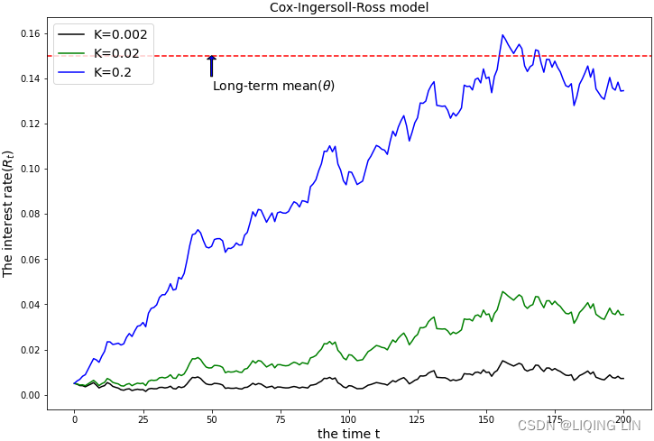With higher levels of speed for mean reversion, K , the process reaches its long-term level of 0.15(the model reverts around the mean, θ=0.15) sooner.
Observe that the CIR interest model does not have negative interest rate values.

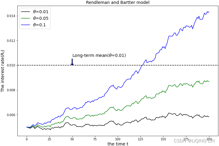
The Rendleman and Bartter model

The Rendleman and Bartter model (Richard J. Rendleman, Jr. and Brit J. Bartter) in finance is a short-rate model describing the evolution of interest rates. It is a "one factor model" as it describes interest rate movements as driven by only one source of market risk. It can be used in the valuation估值 of interest rate derivatives. It is a stochastic asset model.

In the Rendleman and Bartter model, the short-rate process is given as follows:

$\LARGE dr_t = \theta * r_t * dt + \sigma * r_t* \sqrt{dt} * dZ_t$
$\LARGE r_{t+\Delta t} = r_t + dr_t$

$\large r(t)$ Process level at date t
$\large \theta$ Long-term mean of the process
All future trajectories of $\large r(t)$ will evolve around a mean level $\large \theta$ in the long run;
$\large W_t$ is a Wiener process(Standard Brownian motion) under the risk neutral framework modelling the random market risk factor, in that it models the continuous inflow of randomness into the systemhttps://blog.csdn.net/Linli522362242/article/details/125355166
The standard deviation parameter, $\large \sigma$ , determines the volatility of the interest rate and in a way characterizes the amplitude/ˈæmplɪtuːd/ of the instantaneous randomness inflow.
$\large \sigma$ Constant volatility parameter （The spread(range) of the value of $\large r(t)$ ）

$\large \sigma$ :"instantaneous volatility瞬时波动率", measures instant by instant the amplitude of randomness entering the system. Higher $\large \sigma$ implies more randomness

Here, the instantaneous drift is θ*r(t) with an instantaneous standard deviation, σ*r(t). The Rendleman and Bartter model can be thought of as a geometric Brownian motion, akin to a stock price stochastic process that is log-normally distributed(https://blog.csdn.net/Linli522362242/article/details/96593981). This model lacks the property of mean reversion( no K : "speed of reversion回归速度". K characterizes the velocity at which such trajectories will regroup around $\large \theta$ in time; K 表征这些轨迹将在时间 $\large \theta$ 周围重新组合的速度). Mean reversion is a phenomenon where the interest rates seem to be pulled back toward a long-term average level $\large \theta$ .

The following Python code models the Rendleman and Bartter interest-rate process:

import math
import numpy as np

def rendleman_bartter( r0, theta, sigma, T=1, N=10, seed=777 ):
    # r0 : the initial rate of interest at t=0
    # theta : All future trajectories of r(t) will evolve around a 'mean' level 'theta' in the long run
    # sigma : determines the volatility of the interest rate and amplitude(range of r(t)) 
    # T : the period in terms of number of years
    # N : the number of intervals for the modeling process
    # W : a Wiener process(Standard Brownian motion)
    #     modelling the random market risk factor(under the risk neutral framework)
    
    np.random.seed( seed )
    dt = T/float(N)
    
    rates = [r0]                                 # dW = sqrt(dt) * dZ  
    for i in range( N ):                         # Z is a standard normal variable
        dr = theta*rates[-1]*dt + sigma*rates[-1]*math.sqrt(dt)*np.random.normal()
        
        rates.append( rates[-1] + dr )
    # returns a list of time periods and interest rates
    return range(N+1), rates

We will continue to use the example from the previous sections and compare the model.

Assume that the current interest rate is 0.5%, and sigma $\LARGE \sigma$ is 0.05 . We will use a T value of 10 and N of 200 to model the interest rates with different instantaneous drift, theta $\large \theta$ , using values of 0.01 , 0.05 , and 0.1:

%matplotlib inline
import matplotlib.pyplot as plt

fig = plt.figure( figsize=(12,8) )

# r0 : the initial rate of interest at t=0
r0 = 0.005
# sigma : determines the volatility of the interest rate and amplitude(range of r(t)) 
sigma = 0.05
# T : the period in terms of number of years
T = 10
# N : the number of intervals for the modeling process
N = 200    

colors = ['k','g','b']

# theta : All future trajectories of r(t) will evolve around a 'mean' level 'theta' in the long run
theta_list = [0.01, 0.05, 0.1]

for index, theta in enumerate(theta_list):
    N_plus_1, rate_list = rendleman_bartter( r0, theta, sigma, T, N )
    plt.plot( N_plus_1, rate_list,
              label=r'${\theta}$=%s' % theta,
              c = colors[index]
            )

plt.annotate( r'Long-term mean(${\theta}$=0.01)',

              ha='left',

              va='top',

              xytext=(50, 0.01 + 0.001), # The xytext parameter specifies the text position               

              xy=(50, 0.01),     # The xy parameter specifies the arrow's destination 

              arrowprops=dict(facecolor=colors[index], headwidth=10, headlength=4, width=2 ),

              # arrowprops={'facecolor':'blue', 'headwidth':10, 'headlength':4, 'width':2} #OR
              fontsize=14
            )
plt.axhline(y=0.01, ls='--', c=colors[0]) # Long-term mean(theta) of the process

plt.legend( loc='upper left' , fontsize=14)
plt.ylabel('The interest rate$(R_t)$', fontsize=14)
plt.xlabel('the time t', fontsize=14)
plt.title('Rendleman and Bartter model', fontsize=14)
plt.show()

In general, this model lacks the property of mean reversion and grows toward a long-term average level $\large \theta$ .

The Brennan and Schwartz model

The Brennan and Schwartz model is a two-factor model where the short-rate $\large r(t)$ reverts toward a long-term rate as the mean $\large \theta$ , which also follows a stochastic process. (The Brennan and Schwartz model is a two factors model that models the dynamics of the short and long term rates. , ==>
, ==> $\LARGE Cov(dW_{t1}, dW_{t2}) = \rho dt$ http://www.ericbenhamou.net/documents/Encyclo/Brennan%20and%20Schwartz%20_1982_%20model.pdf
OR https://web.mst.edu/~bohner/fim-10/fim-chap6.pdf
)
The short-rate process is given as follows(
The Brennan-Schwartz model is one of the one-factor stochastic differential equation models and it represents the dynamics of the short-rate. It is a "one factor model" as it describes interest rate movements as driven by only one source of market risk): http://trihandika.staff.gunadarma.ac.id/Publications/files/1558/ICREM.pdf
$\LARGE dr_t = K * (\theta - r_t) * dt + \sigma * r_t * dW_t$ ==>
$\LARGE dr_t = K * (\theta - r_t) * dt + \sigma * r_t* \sqrt{dt} * dZ_t$
$\LARGE r_{t+\Delta t} = r_t + dr_t$

$\large r(t)$ Process level at date t,
$\LARGE K * (\theta - r_t)$ is called the drift coefficient
$\LARGE \sigma*r_t$ is called diffusion coefficient(扩散系数) of the process
The drift coefficient $\LARGE K * (\theta - r_t)$ depends on the current value of $\large r(t)$ .
If $\large r(t)$ is less than $\large \theta$ , then the drift coefficient is positive;
if $\large r(t)$ is greater than $\large \theta$ , then it is negative. Thus, the interest-rate tends to revert to its reversion level $\large \theta$ at a rate which depends upon the speed of adjustment K
$\large \theta$ Long-term mean of the process
All future trajectories of $\large r(t)$ will evolve around a mean level $\large \theta$ in the long run;
K Mean-reversion factor
"speed of reversion回归速度". K characterizes the velocity at which such trajectories will regroup around $\large \theta$ in time; K 表征这些轨迹将在时间 $\large \theta$ 周围重新组合的速度
$\large W_t$ is a Wiener process(Standard Brownian motion) under the risk neutral framework modelling the random market risk factor, in that it models the continuous inflow of randomness into the systemhttps://blog.csdn.net/Linli522362242/article/details/125355166
The standard deviation parameter, $\large \sigma$ , determines the volatility of the interest rate and in a way characterizes the amplitude/ˈæmplɪtuːd/ of the instantaneous randomness inflow.
$\large \sigma$ Constant volatility parameter （The spread(range) of the value of $\large r(t)$ ）

$\large \sigma$ :"instantaneous volatility瞬时波动率", measures instant by instant the amplitude of randomness entering the system. Higher $\large \sigma$ implies more randomness

$\large \frac{\sigma^2}{2K}$ : "long term variance". All future trajectories of r will regroup around the long term mean with such variance after a long time.
K and $\large \sigma$ tend to oppose each other:
increasing $\large \sigma$ increases the amount of randomness entering the system, but at the same time increasing K amounts to increasing the speed at which the system will stabilize statistically around the long term mean $\large \theta$ with a corridor(狭长地带,走廊) of variance(OR $\large \sigma^2$ ) determined also by K. This is clear when looking at the long term variance,
increases $\large \frac{\sigma^2}{2K}$ by increasing $\large \sigma$ but decreases $\large \frac{\sigma^2}{2K}$ by increasing K.

It can be seen that the Brennan and Schwartz model is another form of a geometric Brownian motion(https://blog.csdn.net/Linli522362242/article/details/125355166).

import math
import numpy as np

def rendleman_bartter( r0, theta, sigma, T=1, N=10, seed=777 ):
    # r0 : the initial rate of interest at t=0
    # theta : All future trajectories of r(t) will evolve around a 'mean' level 'theta' in the long run
    # sigma : determines the volatility of the interest rate and amplitude(range of r(t)) 
    # T : the period in terms of number of years
    # N : the number of intervals for the modeling process
    # W : a Wiener process(Standard Brownian motion)
    #     modelling the random market risk factor(under the risk neutral framework)
    
    np.random.seed( seed )
    dt = T/float(N)
    
    rates = [r0]                                 # dW = sqrt(dt) * dZ  
    for i in range( N ):                         # Z is a standard normal variable
        dr = theta*rates[-1]*dt + sigma*rates[-1]*math.sqrt(dt)*np.random.normal()
        
        rates.append( rates[-1] + dr )
    return range(N+1), rates

Assume that the current interest rate remains at 0.5%, and the long-term mean level of theta is 0.006. sigma is 0.05 . We will use a T value of 10 and N of 200 to model the interest rates with different speeds of mean reversion, K , using values of 0 2 , 0.02 , and 0.002

%matplotlib inline
import matplotlib.pyplot as plt

fig = plt.figure( figsize=(12,8) )

# r0 : the initial rate of interest at t=0
r0 = 0.005
# K : "speed of Mean-reversion
# theta : All future trajectories of r(t) will evolve around a 'mean' level 'theta' in the long run
theta = 0.006  # long-term mean level of theta
# sigma : determines the volatility of the interest rate and amplitude(range of r(t)) 
sigma = 0.05
# T : the period in terms of number of years
T = 10
# N : the number of intervals for the modeling process
N = 200    
# K : "speed of Mean-reversion

K_list = [0.2, 0.02, 0.002]
colors = ['k','g','b']

for index, K in enumerate(K_list):
    N_plus_1, rate_list =brennan_schwartz( r0, K, theta ,sigma, T, N )
    plt.plot( N_plus_1, rate_list,
              label='K=%s' % K,
              c = colors[index]
            )

plt.axhline(y=theta, ls='--', c='r') # Long-term mean(theta) of the process

plt.annotate( r'Long-term mean(${\theta}$=%s)' % theta,

              ha='center',

              va='top',

              xytext=(50, theta - 0.0001), #The xytext parameter specifies the text position               

              xy=(50, theta),     #The xy parameter specifies the arrow's destination 

              arrowprops=dict(facecolor='blue', headwidth=10, headlength=4, width=2 ),

              #arrowprops={'facecolor':'blue', 'headwidth':10, 'headlength':4, 'width':2} #OR
              fontsize=14
            )


plt.legend( loc='upper left' , fontsize=14)
plt.ylabel('The interest rate$(R_t)$', fontsize=14)
plt.xlabel('the time t', fontsize=14)
plt.title('Brennan and Schwartz model', fontsize=14)
plt.show()

When K is 0.2, the speed of the mean reversion is fastest toward the long-term mean of 0.006.

Bond options

When bond issuers, such as corporations, issue bonds, one of the risks they face is the interest rate risk.

When interest rates(yields) decrease, bond prices increase.
- While existing bondholders will find their bonds more valuable,
- bond issuers, on the other hand, find themselves in a losing position, since they will be issuing higher-interest payments(Coupons) than the prevailing interest rate.
Conversely, when interest rates increase,
- bond issuers are at an advantage, since they are able to continue issuing the same low-interest payments as agreed to on the bond-contract specifications.

To capitalize on利用 interest-rate changes, bond issuers may embed options within a bond. This allows the issuer the right, but not the obligation, to buy or sell the issued bond at a predetermined price during a specified period of time. An American type of bond option allows the issuer to exercise the rights of the option at any point in time during the lifetime of a bond. A European type of bond option allows the issuer to exercise the rights of the option on a specific date. The exact style of the date of exercise行使日期的确切样式 varies from bond option to bond option. Some issuers may choose to exercise the right of the bond option when the bond has been in circulation流通 in the market for over a year. Some issuers may choose to exercise the bond option on one of several specific dates. Regardless of the exercise dates of the bond, you may price the bond with an embedded option, as follows:

Price of bond = price of bond with no option - price of embedded option

The pricing of a bond with no option is fairly straightforward: the present value of the bond to be received at a future date, including all coupon payments. A number of assumptions are to be made about the theoretical interest rates in the future at which the coupon payments may be reinvested.

One such assumption might be the movement of interest rates as implied by short-rate models, which we covered in the preceding section, Short-rate modeling.
Another assumption might be the movement of interest rates within a binomial or trinomial tree. For simplicity, in bond-pricing studies, we will price zero-coupon bonds that will not issue coupons during the lifetime of the bond.

To price an option, one would have to determine available exercise dates. Starting from the future value of the bond, the bond price is compared against the exercise price of the option and traverses back to the present time using a numerical procedurehttps://blog.csdn.net/Linli522362242/article/details/125355166, such as a binomial tree. This price comparison is performed at time points when the bond option may be exercised. With the no-arbitrage theory, accounting for the present excess values of the bond when exercised, we obtain the price of the option. For simplicity, in bond-pricing studies in the later section of this chapter, Pricing callable bond options, we will treat the embedded option of zero-coupon bonds as an American option.

Callable bonds可赎回债券

In an economic condition where there are high interest rates, bond issuers are likely at risk of facing an interest-rate decrease( y, $\large BP = \sum_{T=1}^{nt}\frac{\frac{C}{n}}{(1+\frac{y}{n})^{T}} + \frac{FV}{(1+\frac{y}{n})^{nt}}$

While existing bondholders will find their bonds more valuable(BP ),

) and having to continue to issue higher-interest payments(Coupons) than the prevailing interest rate. As such, they may choose to issue callable bonds. A callable bond contains an embedded agreement to redeem赎回(股票/债券等) the bond at agreed dates. Existing bond holders are considered to have sold a call option to the bond issuer.

In the event that interest rates fall(y, BP) and the corporation has the right to exercise the option to buy back the bond during that period at a specific price(K, a call option's profit=BP- K, while existing bondholders' profits = Coupons + (K - initial_BP) and initial_BP<=par value<=K or a callable price ), they may choose to do so. The company can then issue new bonds at lower interest rates. This also means that the company is able to raise more capital in the form of higher bond prices.
################

A callable bond is a debt instrument in which the issuer reserves the right to return the investor's principal and stop interest payments before the bond's maturity date. Corporations may issue bonds to fund expansion or to pay off other loans. If they expect market interest rates to fall(y, BP), they may issue the bond as callable, allowing them to make an early redemption and secure other financings at a lowered rate. The bond's offering will specify the terms of when the company may recall the note.

A callable—redeemable—bond is typically called at a value that is slightly above the par value of the debt. The earlier in a bond's life span that it is called, the higher its call value will be. For example, a bond maturing in 2030 can be called in 2020. It may show a callable price of 102. This price means the investor receives $1,020 for each $1,000 in face value(par value) of their investment. The bond may also stipulate that the early call price goes down to 101 after a year

Price of bond( Callable bonds holders'cost ) = price of bond with no option - price of embedded option

################

Puttable bonds

Unlike callable bonds, the owner of puttable bonds has the right, but not the obligation, to sell the bond back to the issuer at an agreed price during a certain period. Owners of puttable bonds are considered to have bought a put option from the bond issuer. When interest rates increase(y $\large BP = \sum_{T=1}^{nt}\frac{\frac{C}{n}}{(1+\frac{y}{n})^{T}} + \frac{FV}{(1+\frac{y}{n})^{nt}}$ ), values of existing bonds become less valuable(BP) and puttable bond holders are more incentivized to exercise the right to sell the bond at a higher exercise price(put option's profit= K-BP, existing bondholders' profits = Coupons + put option's profit ). Since puttable bonds are more beneficial to buyers than to the issuers, they are generally less common than callable bonds. Variants of puttable bonds can be found in the form of loan and deposit instruments. A customer who has placed a fixed-rate deposit with a financial institution receives interest payments on specified dates. They are entitled to withdraw the deposit at any time. As such, a fixed-rate deposit instrument can be thought of as a bond with an embedded American put option.

################

A bond is a debt instrument that makes periodic interest payments, known as coupons, to investors. When the bond matures, the investors or lenders receive their principal investment valued at par. It is cost-effective成本效益 for bond issuers to issue bonds with lower yields( y) as this reduces their cost of borrowing. However, to encourage investors to accept a lower yield on a bond, an issuer might embed options that are advantageous to bond investors. One type of bond that is favorable to investors is the put, or puttable, bond.

A put bond is a bond with an embedded put option, giving bondholders the right, but not the obligation, to demand early repayment of the principal from the issuer or a third party acting as an agent for the issuer. The put option on the bond can be exercised upon the occurrence of specified events or conditions or at a certain time or times prior to maturity. In effect, bondholders have the option of "putting" bonds back to the issuer either once during the lifetime of the bond (known as a one-time put bond) or on several different dates.

Bondholders can exercise their options if interest rate levels in the markets increase(y). As there is an inverse relationship between interest rates and bond prices, $\large BP = \sum_{T=1}^{nt}\frac{\frac{C}{n}}{(1+\frac{y}{n})^{T}} + \frac{FV}{(1+\frac{y}{n})^{nt}}$ when interest rates increase, the value of a bond decreases(BP) to reflect the fact that there are bonds in the market with higher coupon rates than what the investor is holding. In other words, the future value of coupon rates becomes less valuable in a rising interest rate environment. Issuers are forced to repurchase the bonds at par, and investors use the proceeds to buy a similar bond offering a higher yield, a process known as bond swap.

Of course, the special advantages of put bonds mean that some yield must be sacrificed. Investors are wiling to accept a lower yield on a put bond than the yield on a straight bond(bond with no option) because of the value added by the put option. Likewise, the price of a put bond is always higher than the price of a straight bond(bond with no option). While a put bond allows the investor to redeem a long-term bond before maturity, the yield generally equals the one on short-term rather than long-term securities.

################

An investor who wishes to borrow money from a bank enters a loan agreement, making interest payments during the lifetime of the agreement until the debt, together with the principal amount and agreed interest(Coupons), is fully repaid. The bank can be considered as buying a put option on a bond. Under certain circumstances, the bank may exercise the right to redeem the full value of the loan agreement.

Thus, the price of puttable bonds can be thought of as follows:

Price of puttable bond = price of bond with no option + price of put option

Price of puttable bond( Puttable bonds holders'cost ) = price of bond with no option + price of put option

Convertible bonds

Convertible bonds are issued by companies and contain an embedded option that allows the holder to convert the bond into a number of shares of common stock. The amount of shares to be converted for a bond is defined as the conversion ratio, which is determined such that the dollar amount of shares is the same as the value of the bond.

Convertible bonds have similarities with callable bonds(
Price of bond( Callable bonds holders'cost ) = price of bond with no option - price of embedded option
). They allow the bond holders to exercise the bond for an equivalent amount of shares at the specified conversion ratio at agreed times. Convertible bonds typically issue lower coupon rates than non-convertible bonds, to compensate for the additional value of the right to exercise.

When convertible bond holders exercise their rights into stocks, the company's debts are reduced. On the other hand, the company's stocks become more diluted/daɪˈluːtɪd/稀释的 as the number of shares in the circulation increases, and the company's stock price is expected to fall.

As the company's stock price increases, convertible bond prices tend to increase.
Conversely, as the company's stock price decreases, convertible bond prices tend to decrease.

################

As an example, let's say Exxon Mobil Corp. (XOM) issued a convertible bond with a $1,000 face value that pays 4% interest(Coupons interest). The bond has a maturity of 10 years and a convertible ratio of 100 shares for every convertible bond.

If the bond is held until maturity, the investor will be paid $1,000 in principal plus $40 in interest for that year. However, the company's shares suddenly spike and are trading at $11 per share. As a result, the 100 shares of stock are worth $1,100 (100 shares x $11 share price), which exceeds the value of the bond. The investor can convert the bond into stock and receive 100 shares, which could be sold in the market for $1,100 in total.

########

Convertible bonds are debt securities that can be converted into a firm’s stock at a pre-specified price. For instance, you might have a convertible bond with a face (or par) value of $1,000 that pays 6 percent interest, or $60(Coupons), each year. The bond matures in five years, at which time the company must pay the $1,000 par value to the bondholder. However, at
the time the bond was issued, the firm gave the bondholder the option of

either collecting the $1,000
or receiving shares of the firm’s stock at a conversion price of $50.

In other words, the bondholder would receive 20 shares ( $20 = \frac{1000}{50}$ , a convertible ratio of 20 shares for every convertible bond). What would you do if you were the bondholder? If the stock were selling for more than $50, then you would want to give up the $1,000 par value and take the stock. Thus, it’s the investor’s choice either to take the $1,000 promised when the bond was issued or to convert the bond into the firm’s stock.

################

Preferred stocks

Preferred stocks are stocks that have bond-like qualities. Owners of preferred stocks have seniority(/ˌsiːnˈjɔːrəti/) of claim on dividend payments over common stocks, which are usually negotiated as a fixed percentage of their par value. Although there is no guarantee of dividend payments, all dividends are paid on preferred stock first over common stock. In certain agreements on preferred stocks, dividends that are not paid as agreed may accumulate until they are paid at a later time. These preferred stocks are known as cumulative.

Prices of preferred stocks typically move in tandem/ˈtændəm/ with同步变动 their common stock. They may have voting rights associated with common shareholders. In the event of bankruptcy, preferred stocks have a first lien优先留置权 of its par value upon liquidation清算.

Pricing a callable bond option

In this section, we will take a look at pricing a callable bond. We assume that the bond to be priced is a zero-coupon paying bond with an embedded European call option. The price of a callable bond can be thought of as follows:

Price of callable bond = price of bond with no option − price of call option

Pricing a zero-coupon bond by the Vasicek model

$BP = \sum_{t=1}^{T}\frac{C}{e^{Rt}} + \frac{PV_{T}}{e^{RT}} = \sum_{t=1}^{T}\frac{C}{e^{Rt}} + \frac{ParVar}{e^{RT}}$ continuously compounded interest rate R or r

$t=1, 1*\Delta t;t=2, 2*\Delta t,t=3, 3*\Delta t,...$

The value of a zero-coupon bond(C=0) with a par value of 1 at time t and a prevailing interest rate, r, is defined as follows:
$P(t)=e^{-rdt}<==BP=e^{-r\Delta t}<==BP=e^{-rt}, 0 \leqslant t \leqslant T$
Since the interest rate, r, is always changing, we rewrite the zero-coupon bond as follows:
$\large P(t,T) = e^{-\int_{t}^{T}r(s)ds}$ , $\large t \leqslant s \leqslant T$ (Similarly to the above, when the short-term interest rate process ( r(t) ) t∈ $\large R_{+}$ is a deterministic function of time)

Now, the interest rate, r, is a stochastic process that accounts for the price of the bond from time t to T, where T is the time to maturity of the zero-coupon bond.

To model the interest rate, r, we can use one of the short-rate models as a stochastic process. For this purpose, we will use the Vasicek model to model the short-rate process.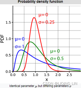

The expectation of a log-normally distributed variable, X, is given as follows:

the arithmetic mean算术平均值 of a log-normally distributed variable X

Taking moments of the log-normally distributed variable X (For any real or complex number s, the s-th moment(s阶矩) of a log-normally distributed variable X is given by):
$\LARGE E\left [ X^s \right ]=E\left [ e^{su} \right ] = e^{su + \frac{s^2\sigma^2 }{2}}$

We obtained the expected value of a log-normally distributed variable, which we will use in the interest-rate process for the zero-coupon bond.

Remember the Vasicek short-rate process model (specifies that the instantaneous interest rate follows the stochastic differential equation(SDE), Under the the risk-neutral probability measure $\large Q$ ):

$\LARGE dr_t = K*(\theta - r_t) *dt + \sigma* \sqrt{dt}* dZ_t$ OR

where

$\large (W_t)_{t\geq 0}$ is a standard $\large Q$ -Brownian motion
$\large K > 0$ is the speed of mean reversion
$\large \theta > 0$ is the long-term value of interest rate
$\large \sigma > 0$ is a constant volatility

where K, θ, σ > 0 and W is a Brownian motion under the risk-neutral measure
$\LARGE dr_t = K \theta dt - K r_t dt + \sigma dw_t$
$\LARGE dr_t + K r_t dt = K \theta dt + \sigma dw_t$ ==>Multiplying both sides by $\LARGE e^{Kt}$ yields
$\LARGE e^{Kt} dr_t + e^{Kt} K r_t dt = e^{Kt} K \theta dt + e^{Kt} \sigma dw_t$
$\large (e^{Kt} * rt) ' = \frac{d}{dt}(e^{Kt} * r_t) = e^{Kt} \frac{d}{dt}(r_t) + r_t \frac{d}{dt}(e^{Kt})$
$\large \frac{d}{dt}(e^{Kt} * r_t) = e^{Kt} \frac{d}{dt}(r_t) + r_t e^{Kt}*K$ ==>Multiplying by $\large dt$ yields
$\large d(e^{Kt} * r_t) = e^{Kt} d(r_t) + r_t e^{Kt}*K*dt$
$\large d(e^{Kt} r_t) = e^{Kt} d(r_t) + Kr_t e^{Kt}dt$
$\LARGE d(e^{Kt} r_t) = e^{Kt} K \theta dt + e^{Kt} \sigma dw_t$ ==> integrating from $\LARGE s$ to $\LARGE t$
$\LARGE \int_{s}^{t} d(e^{Ku} r_u) = K \theta \int_{s}^{t} e^{Ku} du + \sigma \int_{s}^{t} e^{Ku} dw_u$
$\LARGE e^{Kt} r_t - e^{Ks} r_s= K \theta\frac{e^{Kt} - e^{Ks} }{ K } + \sigma \int_{s}^{t} e^{Ku} dw_u$
$\LARGE r_t - e^{K(s-t)} r_s= \theta e^{K(t-t)} - \theta e^{K( s-t) } + \sigma \int_{s}^{t} e^{ K(u-t)} dw_u$

$\LARGE r_t = e^{K(s-t)} r_s + \theta - \theta e^{K( s-t) } + \sigma \int_{s}^{t} e^{ K(u-t)} dw_u$

$\LARGE r_t = r_s e^{K(s-t)} + \theta (1- e^{K( s-t) } ) + \sigma \int_{s}^{t} e^{ K(u-t)} dw_u$
$\LARGE r_t = r_s e^{-K(t-s)} + \theta (1- e^{-K( t-s) } ) + \sigma \int_{s}^{t} e^{- K(t-u)} dw_u$
if $\LARGE s=0$ OR Let 0 ≤ u ≤ t

$\LARGE r_t = r_0 e ^{-Kt} + \theta ( 1 - e^{-Kt} ) + \sigma \int_{0}^{t} e^{K(u-t)} dWu$

$\LARGE r_t = \theta + (r_0 - \theta) e^{-Kt} + \sigma \int_{0}^{t} e^{K(u-t)} dWu$

##################

Since the interest rate, r, is always changing, we rewrite the zero-coupon bond as follows:
$\large P(t,T) = e^{-\int_{t}^{T}r(s)ds}$ , $\large t \leqslant s \leqslant T$ (Similarly to the above, when the short-term interest rate process ( r(t) ) t∈ $\large R_{+}$ is a deterministic function of time)

##################https://web.mst.edu/~bohner/fim-10/fim-chap4.pdf

Using the characteristic equation and the interest-rate movements of the Vasicek model, we can rewrite the zero-coupon bond price in terms of expectations:

In the one-factor Vasicek model, the short-term interest rate $\large r_t$ is modeled as a mean reverting Gaussian stochastic process on a probability space $\large \left ( \Omega,F,P \right )$ equipped with aa filtration $\large (F_t)_{t\geq 0}$
Consider a frictionless and no-arbitrage无摩擦且无套利 financial market which consists of a bank account $\large A_t$ with its price process given by $\large dA_t = r_t A_t dt$ and a T-maturity default-free, zero coupon bond $\large P(t,r,T) = P_t =P(t)$ with its no-arbitrage price at time t given by

$\large P(t,r,T) = E{_{Q}}^{t}\left [ e^{-\int_{t}^{T}r(u)du} \right | Ft] = E_{Q}\left [ e^{-\int_{t}^{T}r(s)ds} \right]=P(t)$ $\large 0 \leqslant t \leqslant T$ where $\large E_Q$ is the expectation value under the risk-neutral probability measure $\large Q$ . Vasicek provides the explicit form of the zero-bond as follows:
$\large P(t,T) = P(t,r,T) = A(t,T) e^{-r(t) B(t,T)}$ (2.3)
$\LARGE B(t,T) = \frac{1-e^{-K(T-t)}}{K}$ OR
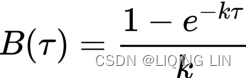
$\large A(t,T) = e^{ ( \theta - \frac{ \sigma^2}{2K^2} ) ( B(t,T)-(T-t) ) - \frac{\sigma ^2}{4K} B^2(t,T) }$ OR
From (2.3), we are easy to obtain the following partial differential equation (PDE):

$\large \frac{\partial P_t}{\partial t} + K(\theta -r)\frac{\partial P_t}{\partial r} + \frac{1}{2}\sigma^2\frac{\partial^2 P_t}{\partial r^2} - rP_t =0$
with terminal condition $\large P(T,r,T)=1$ .
https://downloads.hindawi.com/archive/2009/215163.pdf

https://web.mst.edu/~bohner/fim-10/fim-chap4.pdf

http://public.kenan-flagler.unc.edu/faculty/lundblac/bcrp/vasicek77.pdf https://quant.stackexchange.com/questions/45216/finding-bt-in-the-vasicek-model-relating-to-the-bond-equation-more-specifcall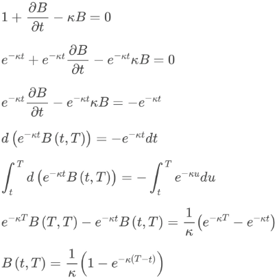

The Python implementation of the zero-coupon bond price is given in the exact_zcb function:

# Pricing a zero-coupon bond by the Vasicek model
import numpy as np
import math

# zcb: Zero_Coupon_Bond
def exact_zcb( theta, Kappa, sigma, t_T, r0=0. ):
    # r0 : the initial rate of interest at t=0
    # Kappa : "speed of Mean-reversion
    # theta : All future trajectories of r(t) will evolve around a 'mean' level 'theta' in the long run
    # sigma : determines the volatility of the interest rate and amplitude(range of r(t)) 
    # T : the period in terms of number of years
       
    # 0<= t <=T
    B = ( 1-np.exp(-Kappa*t_T ) ) / Kappa
    A = np.exp( ( theta - (sigma**2)/(2*Kappa**2) ) *\
                ( B - t_T ) - (sigma**2)/(4*Kappa)*(B**2)
              )
    return A * np.exp( -r0*B )

For example, we are interested in finding out the prices of zero-coupon bond prices for a number of maturities. We model the Vasicek short-rate process with a theta('mean') value of 0.5, kappa value of 0.02 , sigma value of 0.03 , and an initial interest rate, r0 , of 0.015. Plugging these values into the exact_zcb function, we obtain zero-coupon bond prices, for the time period from 0 to 25 years with intervals of 0.5 years, and plot out the graph:

# r0 : the initial rate of interest at t=0
r0=0.015
# Kappa : "speed of Mean-reversion
Kappa = 0.2
# theta : All future trajectories of r(t) will evolve around a 'mean' level 'theta' in the long run
theta = 0.5
# sigma : determines the volatility of the interest rate and amplitude(range of r(t)) 
sigma = 0.03
# T : the period in terms of number of years

Ts = np.r_[0.0:25.5:0.5]


zcbs= [ exact_zcb( theta, Kappa, sigma, t, r0 )
        for t in Ts
      ]

print(zcbs)

%matplotlib inline
import matplotlib.pyplot as plt

fig = plt.figure( figsize=(12,8) )

plt.title( "Zero coupon Bond (ZCB) Values by Time" )
plt.plot( Ts, zcbs, label='ZCB')
plt.ylabel( "Value ($)" )
plt.xlabel( "Time in years" )
plt.legend()
plt.grid(True)
plt.show()

The value of early exercise

Issuers of callable bonds may redeem the bond at an agreed price, as specified in the contract. To price such a bond, the discounted early-exercise values can be defined as follows:

Here,

k is the price ratio of the strike price to the par value and
r is the interest rate for the strike price.

The Python implementation of the early-exercise option can then be written as follows:

import numpy as np

def exercise_value( K, R, t ):
    # k is the price ratio of the strike price to the par value
    # R is the interest rate for the strike price.
    return K * np.exp(-R*t)

In the preceding example, we are interested in valuing a call option with a strike ratio of 0.95 and an initial interest rate of 1.5%. We can then plot the values as a function of time and superimpose them onto a graph of zero-coupon bond prices to give us a better visual representation of the relationship between zero-coupon bond prices and callable bond prices:

# r0 : the initial rate of interest at t=0
r0=0.015
# Kappa : "speed of Mean-reversion
Kappa = 0.2
# theta : All future trajectories of r(t) will evolve around a 'mean' level 'theta' in the long run
theta = 0.5
# sigma : determines the volatility of the interest rate and amplitude(range of r(t)) 
sigma = 0.03
# T : the period in terms of number of years

Ts = np.r_[0.0:25.5:0.5]


zcbs= [ exact_zcb( theta, Kappa, sigma, t, r0 )
        for t in Ts
      ]

# k is the price ratio of the strike price to the par value
k=0.95

Ks = [ exercise_value( k, r0, t)
       for t in Ts
     ]

print(Ks)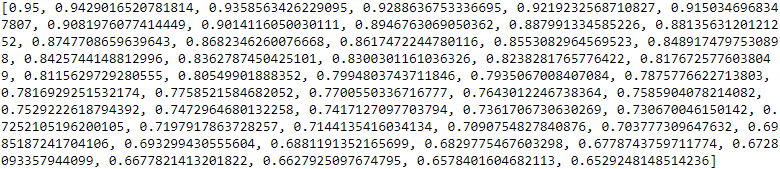

%matplotlib inline
import matplotlib.pyplot as plt

fig = plt.figure( figsize=(12,8) )

plt.title( "Zero Coupon Bond (ZCB) and Strike (K) Values by Time" )

plt.plot( Ts, zcbs, label='ZCB')
plt.plot( Ts, Ks, label='K', linestyle="--", marker=".")

plt.ylabel( "Value ($)" )
plt.xlabel( "Time in years" )
plt.legend()
plt.grid(True)
plt.show()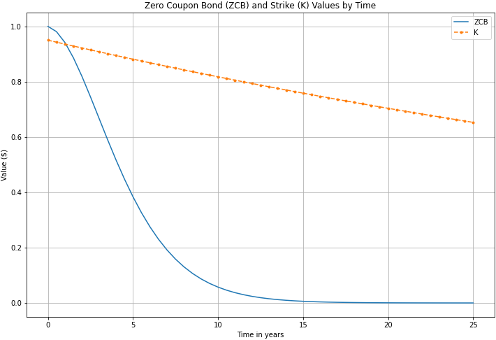

From the preceding graph, we can approximate the price of callable zero-coupon bond prices. Since the bond issuer owns the call, the price of the callable zero-coupon bond can be stated as follows:

This callable bond price is an approximation, given the current interest-rate level. The next step would be to treat early-exercise by going through a form of policy iteration, which is a cycle used to determine optimum early-exercise values and their effect on other nodes, and check whether they become due for an early exercise. In practice, such an iteration only occurs once.

Policy iteration by finite differences

So far, we have used the Vasicek model in our short-rate process to model a zero-coupon bond. We can undergo policy iteration by finite differences to check for early-exercise conditions and their effect on other nodes. We will use the implicit method of finite differences for the numerical pricing procedure, as discussed in https://blog.csdn.net/Linli522362242/article/details/125355166, Numerical Procedures for Pricing Options.

Let's create a class named VasicekCZCB , which will incorporate all the methods used to implement the pricing of callable zero-coupon bonds by the Vasicek model. The class with its constructor definition is given as follows:

class VasicekCZCB:
    
    def __init__(self):
        # the 'inverse' normal cumulative distribution function
        # https://blog.csdn.net/Linli522362242/article/details/103646927
        # confidence (interval)= 0.95 ==>(1-confidence)/2 = 0.025 ==>1-0.025=0.975
        # P(z<Z?) = 0.975 ==> Z?=1.96
        self.norminv = st.distributions.norm.ppf
        # the normal Cumulative Distribution Function
        # https://blog.csdn.net/Linli522362242/article/details/125662545
        # P(z<1.96) ==> 0.975 # probability(area) under the curve
        self.norm = st.distributions.norm.cdf

In the constructor, the norminv and norm variable is made available to all methods that
require the computation of the inverse normal cumulative distribution function and the
normal cumulative distribution function of SciPy, respectively.

Add the vasicek_limits() method to compute the minimum and maximum of the Vasicek interest rate process by a normal distribution process. The expected value of the short-rate process, r(t) , under the Vasicek model is given as follows:
https://web.mst.edu/~bohner/fim-10/fim-chap4.pdf
Let 0 ≤ s ≤ t ≤ T. The short rate in the Vasicek model is given by
$\large r_t = r_s e^{-K(t-s)} + \theta (1- e^{-K( t-s) } ) + \sigma \int_{s}^{t} e^{- K(t-u)} dw_u$
and is, conditionally on $\large F(s)$ , normally distributed with $\large E(r_t|F(s)) = r_s e^{ -K(t-s) } + \theta (1-e^{-K(t-s)} )$
if s=0, then
$\large E(r_t|F(0)) = r_0 e^{ -K(t-0) } + \theta (1-e^{-K(t-0)} )$
$\large E(r_t|F(0)) = r_0 e^{ -Kt } + \theta (1-e^{-Kt} )$
$\large E(r_t|F(0)) = \theta + ( r_0 - \theta ) e^{-Kt} )$
The variance is defined as follows:
$\large Var( r_t | F(s) ) = \frac{\sigma^2}{2K}( 1-e^{ -2K(t-s) } )$
if s=0, then
$\large Var( r_t | F(0) ) = \frac{\sigma^2}{2K}( 1-e^{ -2K(t-0) } )$
$\large Var( r_t | F(0) ) = \frac{\sigma^2}{2K}( 1-e^{ -2Kt } )$
This method returns a tuple of the minimum and maximum interest-rate level as defined by the probability for the normal distribution process, and is written as follows:

    # to compute the minimum and maximum of the Vasicek interest rate process 
    # by a normal distribution process.
    def vasicek_limits(self, r0, sigma, Kappa, theta, T, prob=1e-6):
        
        E_rt = theta + (r0-theta)*math.exp(-Kappa*T )
        variance = (sigma**2)*T if Kappa==0 else \
                    (sigma**2)/( 2*Kappa )*( 1-math.exp(-2*Kappa*T) )
        stddev = math.sqrt(variance)
        # Compute the inverse of cdf values evaluated 
        # at the probability values in 'prob' 
        # for the normal distribution with 'mean/mu/theta
        # and standard deviation 'sigma'
        # ppf(q, loc=0, scale=1) = ppf(prob, theta, sigma)
        r_min = self.norminv( prob, E_rt, stddev )   # P(Z<=r_min) = prob
        r_max = self.norminv( 1-prob, E_rt, stddev ) # P(Z>=r_max) = 1-prob
        
        #####################
        z = np.linspace(-4*stddev,8*stddev,1000)
        fz = st.distributions.norm.pdf(z, E_rt, stddev)
        plt.plot(z, fz, label='f(z)')
#         plt.axvline(r_min, color='blue', label='z>=r_min')
#         plt.axvline(r_max, color='red', label='z<=r_max')
        plt.fill_between(z, fz, 0, where= (r_min<z) & (z<r_max) )
        plt.annotate( 'r_min={:.4f}'.format(r_min),
            ha='center',
            va='bottom',

            xytext=(r_min, 1), #The xytext parameter specifies the text position               
            xy=(r_min, 0),     #The xy parameter specifies the arrow's destination 

            arrowprops=dict(facecolor='blue', headwidth=5, headlength=3, width=1 ),
            #arrowprops={'facecolor':'blue', 'headwidth':10, 'headlength':4, 'width':2} #OR
            fontsize=10
            )
        plt.annotate( 'r_max={:.4f}'.format(r_max),
            ha='center',
            va='bottom',

            xytext=(r_max, 1), #The xytext parameter specifies the text position               
            xy=(r_max, 0),     #The xy parameter specifies the arrow's destination 

            arrowprops=dict(facecolor='blue', headwidth=5, headlength=3, width=1 ),

            #arrowprops={'facecolor':'blue', 'headwidth':10, 'headlength':4, 'width':2} #OR
            fontsize=10
        )
        
        plt.annotate( r'$\theta$={:.2f}'.format(E_rt),
            ha='center',
            va='bottom',

            xytext=(E_rt, 1), #The xytext parameter specifies the text position               
            xy=(E_rt, 0),     #The xy parameter specifies the arrow's destination 

            arrowprops=dict(facecolor='blue', headwidth=5, headlength=3, width=1 ),

            #arrowprops={'facecolor':'blue', 'headwidth':10, 'headlength':4, 'width':2} #OR
            fontsize=10
        )
        
        plt.text( 
                E_rt, 6, #The xytext parameter specifies the text position               
                'P(r_min<= (Z={:.6f}) <=r_max)'.format(1-2*prob),
                fontsize=10,
                horizontalalignment = 'center'
        )
        plt.xlabel('Z-score')
        plt.title('$E(r_t)$, stddev from Vasicek model, prob={} to get r_min and rmax'.format(prob))
        plt.legend()
        #####################
        
        return (r_min, r_max)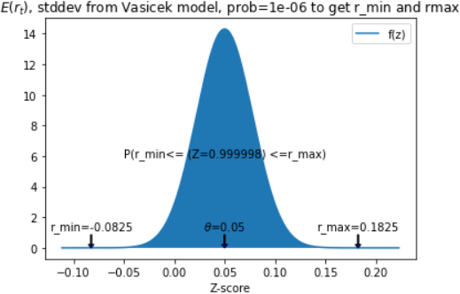

Add the calculate_N() method, which is used by the vasicek_params() method to compute the grid size parameter, N. This method is written as follows:

    # to compute the grid size parameter, N
    def calculate_N( self, max_structure_const, 
                     dt, sigma, r_max, r_min 
                   ):
        N = 0
        # sigma : "instantaneous volatility", 
        # measures instant by instant the amplitude of randomness entering the system.
        #          The spread(range) of the value of r_t
        while True:
            N += 1
            # constraints: dt * sigma**2 / (dr)**2 <= max_structure_const
            grid_structure_interval = dt*sigma**2/\
                    ( (r_max-r_min)/float(N) )**2
                # dr = dS = (r_max-r_min)/float(N)
                # at a time point: n = sigma**2 / (dr)**2 = big square/small square
                # n * dt : over time dt
            # grid_struct_const is the maximum threshold of dt movement 
            # that determines N in the calculate_N() method;    
            if grid_structure_interval > max_structure_const:
                break

        return N

Add the vasicek_params() method to compute the implicit scheme parameters for the Vasicek model. It returns a tuple of r_min , dr , N , and dt . If no value is supplied to r_list , values of r_min to r_max will be automatically generated by the vasicek_limits() method as a function of prob following a normal distribution. This method is written as follows:

    # to compute the implicit scheme parameters for the Vasicek model.
    def vasicek_params( self, r0, M, sigma, Kappa, theta, T,
                        prob, grid_struct_const=0.25, r_list=None
                      ):
        if r_list is not None:
            (r_min, r_max) = ( r_list[0], r_list[-1] )
        else:
            (r_min, r_max) = self.vasicek_limits( r0, sigma, Kappa, 
                                                  theta, T, prob )
        
        dt = T/float(M) # 0<=t<=T
        
        N = self.calculate_N( grid_struct_const, dt, sigma, r_max, r_min )
        dr = (r_max-r_min)/(N-1)
        
        return (r_min, dr, N, dt )

Add the exercise_call_price() method, which returns the discounted value of the strike price as a ratio, written as follows:
discounted early exercise value
Here, k is the price ratio of the strike price to the par value(=1)
and r is the interest rate for the strike price.
```
    # Returns the discounted value of the strike price
    def exercise_call_price( self, R, ratio, tau ):
        K_from_maturity_to_t = ratio*np.exp(-R*tau)
        return K_from_maturity_to_t # 0<= s <=T and T-s=t
```

Add the vasicek_diagonals() method, which returns the diagonals of the implicit scheme of finite differences, where:

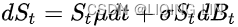
Equation 12-2. Stochastic differential equation in Black-Scholes-Merton setup==>
For the implicit method the Black-Scholes-Merton partial differential equation,
$\large rf = \frac{\partial f}{\partial t} + rS\frac{\partial f}{\partial S} + \frac{1}{2}\sigma^2S^2\frac{\partial^2 f}{\partial S^2}$ ==>
$\large rf_{i,j} = \frac{f_{i,j+1}-f_{i,j}}{d t} + ridS\frac{f_{i+1,j}-f_{i-1,j}}{2 dS} + \frac{1}{2}\sigma^2(idS)^2\frac{f_{i+1,j}-2f_{i,j}+f_{i-1,j}}{(dS)^2}$
$\LARGE f_{i,j+1} = \alpha_if_{i-1,j} + b_i f_{i,j} + c_i f_{i+1,j}$

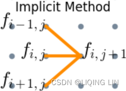
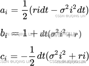
https://blog.csdn.net/Linli522362242/article/details/125355166
https://downloads.hindawi.com/archive/2009/215163.pdf
https://econwpa.ub.uni-muenchen.de/econ-wp/fin/papers/9702/9702003.pdf
$\large \frac{\partial P_t}{\partial t} + K(\theta -r)\frac{\partial P_t}{\partial r} + \frac{1}{2}\sigma^2\frac{\partial^2 P_t}{\partial r^2} - rP_t =0$
$\large rP_t = \frac{\partial P_t}{\partial t} + K(\theta -r)\frac{\partial P_t}{\partial r} + \frac{1}{2}\sigma^2\frac{\partial^2 P_t}{\partial r^2}$
$\large sub-diagnoals, a=K(\theta-r_i)\frac{1}{2dr}dt - \frac{1}{2}\sigma^2\frac{1}{dr^2}dt$
$\large diagnoals, b=1 + r_idt + \sigma^2\frac{1}{dr^2}dt$
$\large super-diagnoals, c=-K(\theta-r_i)\frac{1}{2dr}dt - \frac{1}{2}\sigma^2\frac{1}{dr^2}dt$
Here, $\large a$ is a list for the sub-diagonals,
b is a list for the diagonal, and
c is the super-diagonal of the matrix.
The boundary conditions are implemented using Neumann boundary conditions. This method is written as follows:
$\large \begin{bmatrix} b_1 & c_1 & 0 & 0\\ a_2 & b_2 & \ddots & 0\\ 0 & \ddots & \ddots & c_{n-1}\\ 0 & 0 & a_n & b_n\\ \end{bmatrix} \begin{bmatrix} x_1\\ x_2\\ \vdots \\ x_n \end{bmatrix} = \begin{bmatrix} d_1\\ d_2\\ \vdots \\ d_n \end{bmatrix}$

    def vasicek_diagonals( self, sigma, kappa, theta, 
                           r_min, dr, N, dtau
                         ):
        r_list = np.r_[0:N]*dr + r_min
        # a_i
        subdiagonals = kappa*(theta-r_list)*dtau/(2*dr) -\
                        0.5*(sigma**2)*dtau/(dr**2)
        # b_i
        diagonals = 1 + r_list*dtau + sigma**2*dtau/(dr**2)
        # c_i
        superdiagonals = -kappa*(theta-r_list)*dtau/(2*dr) -\
                        0.5*(sigma**2)*dtau/(dr**2)
        
        # Implement boundary conditions.
        if N > 0:                      # N=1
            v_sub_d0 = subdiagonals[0] # a0
                                       # c0 = c0-a0 = -K*(theta-r0)*dt/dr
            superdiagonals[0] = superdiagonals[0]-subdiagonals[0]
            diagonals[0] += 2*v_sub_d0 # b0 += 2*a0 = K*(theta-r0)*dt/dr - sigma^2*dt/dr^2
            subdiagonals[0] = 0        # a0 = 0     = 0

        if N > 1:
            v_super_d_last = superdiagonals[-1] # cn
                                                # cn=cn-an = -K*(theta-rn)*dt/dr
            superdiagonals[-1] = superdiagonals[-1] - subdiagonals[-1]
            diagonals[-1] += 2*v_super_d_last   # bn += 2*cn
            superdiagonals[-1] = 0              # cn = 0
        
        return (subdiagonals, diagonals, superdiagonals)

Add the tridiagonal_solve() method, which implements the Thomas algorithm to solve tridiagonal systems of equations. The systems of equations may be written as follows:

This equation is represented in matrix form:
Here,
- $\LARGE a$ is a list for the sub-diagonals,
- $\LARGE b$ is a list for the diagonal, and
- $\LARGE c$ is the super-diagonal of the matrix.
- The Thomas algorithm is a matrix algorithm for solving tridiagonal systems of equations using a simplified form of Gaussian elimination. Further information can be found at Tridiagonal Matrices. http://www.industrial-maths.com/ms6021_thomas.pdf
  $\LARGE a_i x_{i-1} + b_i x_i + c_i a_i x_{i+1} = d_i$
  where $\large a_1 = 0$ and $\large c_n = 0$ .
  The Thomas algorithm is an efficient way of solving tridiagonal matrix systems. It is based on LU decomposition in which the matrix system $\large Mx=d$ is rewritten as $\large LUx = d$ where L is a lower triangular matrix and U is an upper triangular matrix.
  ###########################
  LU   https://blog.csdn.net/Linli522362242/article/details/125546725
  We will look at a simple example and write out the row operations.
  
  L : row operation and constraint : column_index= row_index
  
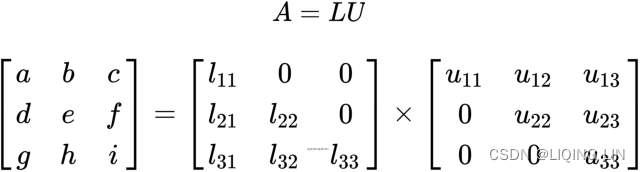
  We will look at a simple example and write out the row operations.
  The system can be efficiently solved by setting $\large Ux = \rho$ and then solving first $\large L \rho= d$ for $\large \rho$ and then $\large Ux = \rho$ for $\large x$ . The Thomas algorithm consists of two steps. In Step 1 decomposing the matrix into M = LU ( $\large LUx = d$ ) and solving $\large L \rho= d$ are accomplished in a single downwards sweep,
  #########
  $\large A\vec{x} = \vec{b}$ $\large M\vec{x} = \vec{d}$
  $\large LU\vec{x} = \vec{b}$    $\large LU\vec{x} = \vec{d}$
  $\large L(U\vec{x}) = \vec{b}$    $\large L(U\vec{x}) = \vec{d}$
  $\large L(\vec{d}) = \vec{b}$ and $\large U\vec{x} = \vec{d}$    $\large L(\vec{\rho}) = \vec{d}$ and $\large U\vec{x} = \vec{\rho}$
  
  we should replace the $\large Ld = b$ with Lρ = d in the following picture
  
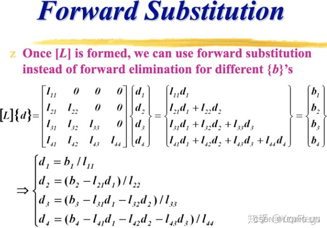
  Ld = b ==>d be replaced with Lρ = d ==> ρ
  
  taking us straight from $\large Mx = d$ to Ux = ρ. In step 2 the equation $\large U\vec{x} = \vec{\rho}$ is solved for x in an upwards sweep.
  
  we should replace the $\large Ux = d$ with Ux = ρ in the following picture
  Ux = d ==>x be replaced with Ux = ρ ==> x
  ###########################http://www.industrial-maths.com/ms6021_thomas.pdf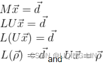
  https://www.cnblogs.com/wft1990/p/5947162.html
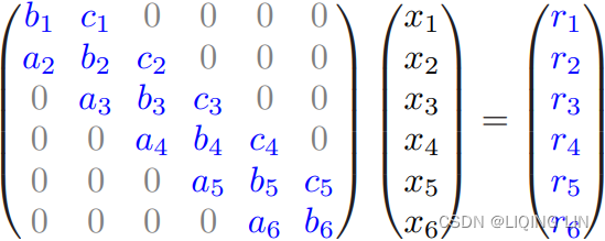
- In the first stage the matrix equation $\large M\vec{x} = \vec{d}$ (OR $\large LU\vec{x} = \vec{d}$ ) is converted to the form $\large U\vec{x} = \vec{\rho}$ . Initially the matrix equation looks like:
  $\large \vec{d} = [r_1, r_2, r_3, r_4,r_5,r_6]$
  STAGE 1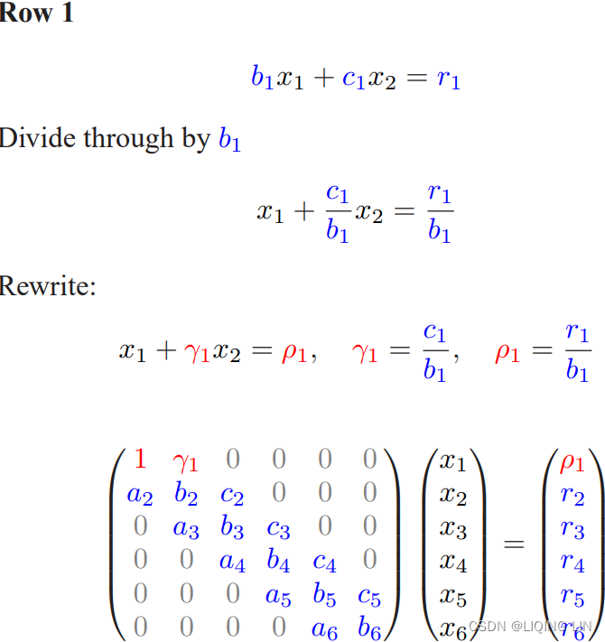
  
  ==>
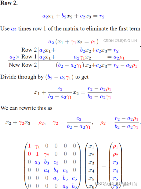
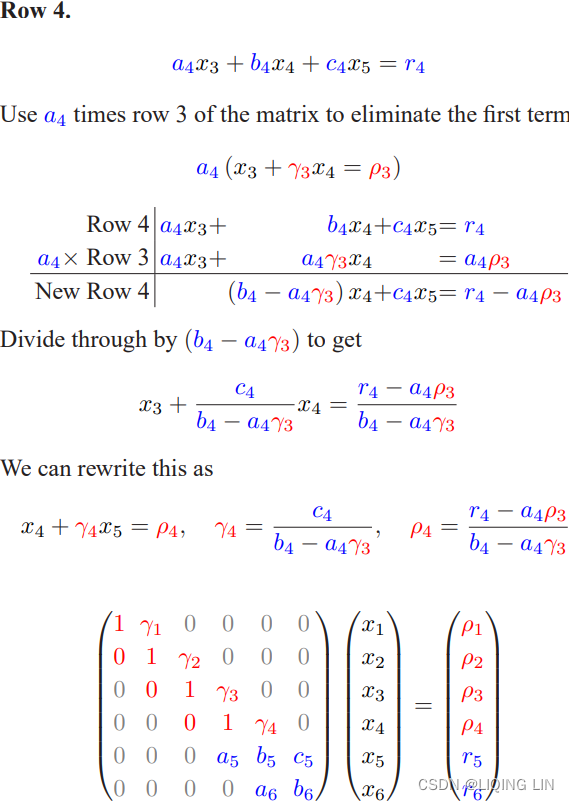
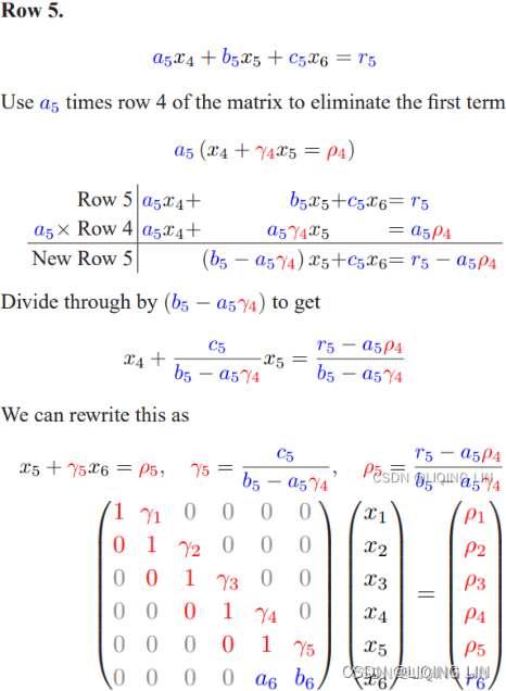
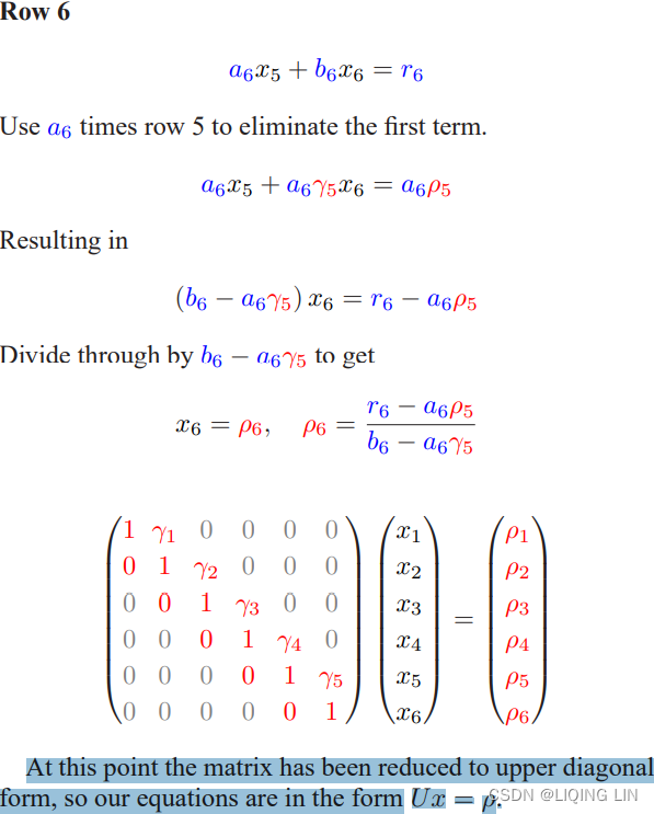  $\large M\vec{x} = \vec{d}$ ==> $\large U\vec{x} = \vec{\rho}$
  STAGE 2
  The matrix equation is now in a form which is trivial to solve for x. We start with the last row and work our way up. The final equation is already solved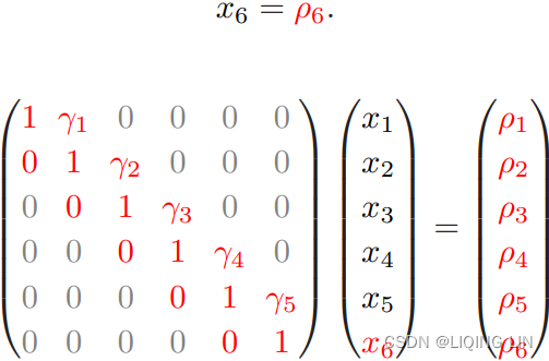
  
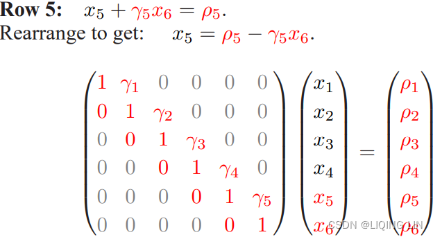
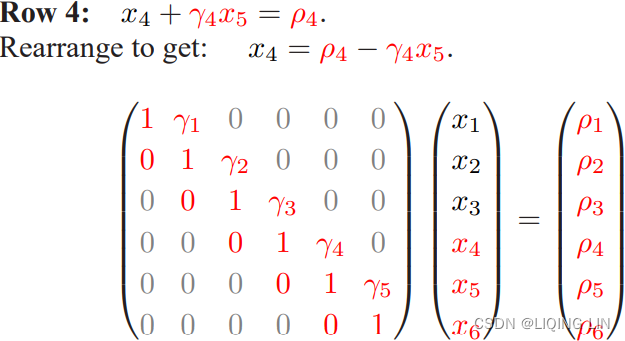
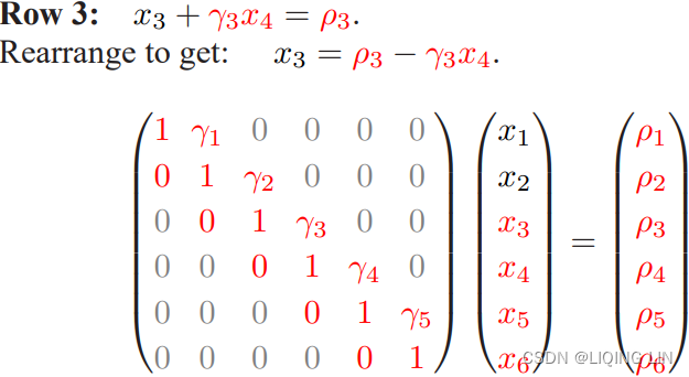
  At this point x, the solution to the matrix equation, is fully determined.and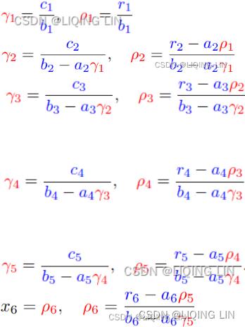
- The Thomas algorithm is used because it is fast and because tridiagonal matrices often occur in practice. (This argument is slightly circular because people often manipulate the problems they are working on to reduce them to solving a tridiagonal matrix problem.) Although it is rare, the algorithm can be unstable if $\large b_i - a_i \gamma_{i-1}$ is zero or numerically zero for any $\large i$ . This
  will occur if the tridiagonal matrix is singular
  (A singular matrix is a square matrix if its determinant行列式 is 0. i.e., a square matrix A is singular if and only if det A = 0. We know that the inverse of a matrix A is found using the formula = (adj A) / (det A)https://blog.csdn.net/Linli522362242/article/details/125546725). Here det A (the determinant of A) is in the denominator. We are aware that a fraction is NOT defined if its denominator is 0. Hence is NOT defined when det A = 0. i.e., the inverse of a singular matrix is NOT defined. i.e., there does not exist any matrix B such that AB = BA = I (where I is the identity matrix).
  ),
  but in rare cases can occur if it is non-singular.
  The condition for the algorithm to be stable is for all $\large i$ . The matrix problems which result from the discretisation of partial differential equations nearly all satisfy this criterion由偏微分方程离散化产生的矩阵问题几乎都满足这个标准
  
  If the algorithm is numerically unstable then you must rearrange the equations: known as pivoting.https://blog.csdn.net/Linli522362242/article/details/125546725 Standard LU decomposition algorithms for full or banded matrices include pivoting. (But first you should check to make sure you have not made a mistake in formulating the problem.)https://www.webpages.uidaho.edu/~barannyk/Teaching/LU_factorization_tridiagonal.pdf
  A = LU
  
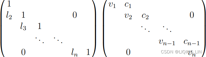
  Structure of Tri-diagonal Matrix
  The LU decomposition algorithm for solving this set is
  http://faculty.washington.edu/finlayso/ebook/algebraic/advanced/LUtri.htm
  To determine L, U:
  
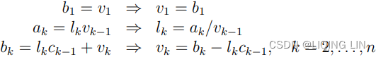
  To solve Ly = f (Lp = d):
  
  To solve Uu = y (Ux=y):
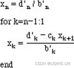
```
    # (a,b,c,d) : (subdiagonal, diagonal, superdiagonal, v_old)
    def tridiagonal_solve(self, a, b, c, d):
        n = len(a)  # Number of equations
        ak, bk, ck, dk = map(np.array, (a, b, c, d))  # Copy the array
        # Ax=LUx=d and A: Matrix composed of all (lk[], bk[] and ck[])
        # d : Matrix of all dk[]
        for k in range(1, n):
            # To determine L, U
            lk = ak[k]/bk[k-1]  # L = Matrixcomposed of all lk[] and identity matrix
            bk[k] -= lk*ck[k-1] # U = Matrix composed of all (bk[] and ck[])
            #ck[k] -= 0 # all values above c[k] are all 0
            # To solve Lp = d ==> p :       Forward Substitution                                
            dk[k] -= lk*dk[k-1] # p[1]=1 && lp[k-1]+1*p[k]=d[k] ==> p[k]=(d[k]-lp[k-1] )/1
                                #                                   p[k] = d[k]-= lp[k-1]
        xk = ak    
        # LUx=d ==> L(Ux)=d ==> Lp=d ==>p and p[k]=d[k] 
        #                x <== Ux=p <== p and know U
        
        # Back Substitution
        xk[-1] = dk[-1]/bk[-1]

        for k in range(n-2, -1, -1):
            xk[k] = (dk[k]-ck[k]*xk[k+1])/bk[k]

        del bk, ck, dk  # Delete variables from memory

        return xk
```

Add the check_exercise() method, which returns a list of Boolean values, indicating the indices suggesting optimum payoff from an early exercise. This method is written as follows:
```
    def check_exercise(self, V, eex):
        return V > eex
```

Add the vasicek_policy_diagonals() method, which is being called by the policy-iteration procedure that updates the sub-diagonals, diagonals, and super-diagonals for one iteration. In indices, where an early exercise is carried out, the sub-diagonals and super-diagonals will have these values set to 0 and the remaining values on the diagonals. The method returns comma-separated values of the new sub-diagonal, diagonal, and super-diagonal values. This method is written as follows:

    def vasicek_policy_diagonals(self, subdiagonal, diagonal,
                                 superdiagonal, v_old,
                                 v_new, eex):
        has_early_exercise = self.check_exercise(v_new, eex)
        subdiagonal[has_early_exercise] = 0
        superdiagonal[has_early_exercise] = 0
        policy = v_old/eex
        policy_values = policy[has_early_exercise]
        diagonal[has_early_exercise] = policy_values
        return (subdiagonal, diagonal, superdiagonal)

Add the iterate() method, which implements the implicit scheme of finite differences by performing a policy iteration, where each cycle involves solving the tridiagonal systems of equations, calling the vasicek_policy_diagonals() method to update the three diagonals, and returns the callable zero-coupon bond price if there are no further early-exercise opportunities. It also returns the number of policy iterations performed.

    def iterate( self, subdiagonal, diagonal, superdiagonal,
                 v_old, eex, max_policy_iter=10
               ):
        v_m_plus1 = v_old
        v_m = v_old
        change = np.zeros(len(v_old))
        prev_changes = np.zeros(len(v_old))

        iterations = 0
        while iterations <= max_policy_iter:
            iterations += 1

            v_m_plus1 = self.tridiagonal_solve(subdiagonal, 
                                diagonal, superdiagonal, v_old
                             )
            subdiagonal, diagonal, superdiagonal = \
                self.vasicek_policy_diagonals(
                    subdiagonal, diagonal, superdiagonal, 
                    v_old,
                    v_m_plus1, eex)

            is_eex = self.check_exercise(v_m_plus1, eex)
            change[is_eex] = 1

            if iterations > 1:
                change[v_m_plus1 != v_m] = 1

            is_no_more_eex = False if True in is_eex else True
            if is_no_more_eex:
                break

            v_m_plus1[is_eex] = eex[is_eex]
            changes = (change == prev_changes)

            is_no_further_changes = all((x == 1) 
                                        for x in changes
                                       )
            if is_no_further_changes:
                break

            prev_changes = change
            v_m = v_m_plus1

        return v_m_plus1, iterations-1

Add the vasicek_czcb_values() method as the point of entry to begin the pricing process. This method returns a list of evenly-spaced short-rates and a list of option prices,
- The r0 variable is the short-rate at time t=0;
- R is the strike zero rate for the bond price;
- ratio is the strike price per par value of the bond;
- T is the time to maturity;
- sigma $\large \sigma$ is the volatility of the short-rate, r;
- Kappa $\large K$ is the rate of mean reversion;
- theta $\large \theta$ is the mean of the short-rate process;
- M is the number of steps in the finite differences scheme
- prob is the probability on the normal distribution curve used by the vasicek_limits method later to determine short-rates;
- max_policy_iter is the maximum number of policy iterations used to find early-exercise nodes;
- grid_struct_const is the maximum threshold of dt movement that determines N in the calculate_N() method;
- and r_list is the list of interest rates from which the short-rate process follows

   # This method returns a list of evenly-spaced short-rates 
    # and a list of option prices, 
    def vasicek_czcb_values( self, r0, R, ratio, T, sigma, Kappa, theta,
                             M, prob=1e-6, max_policy_iter=10, 
                             grid_struct_const=0.25, r_list=None
                           ):
        '''
        r0 : the short-rate at time t=0;
        R : the strike zero rate for the bond price;
        ratio : the strike price per par value of the bond;
        T : the time to maturity;
        sigma : the volatility of the short-rate, r;
        Kappa : the rate of mean reversion;
        theta : the mean of the short-rate process;
        M : the number of steps in the finite differences scheme used by
            the vasicek_limits method later to determine short-rates;
        max_policy_iter : the maximum number of policy iterations used to
                          find early-exercise nodes;
        grid_struct_const : the maximum threshold of dt movement that
                            determines N in the calculate_N() method;
        r_list : the list of interest rates from which the short-rate process follows
        '''
        (r_min, dr, N, dtau) = self.vasicek_params( r0, M, sigma, kappa, theta,
                                                    T, prob, 
                                                    grid_struct_const, r_list
                                                  )
        # N : N rate levels
        # np.r_[0:N] : time step index [0:N-1]
        r_list = np.r_[0:N]*dr + r_min
        v_m_plus1 = np.ones(N)

        # M is the number of steps in the finite differences scheme
        for i in range(1, M+1):
            # K:at step i, the discounted value of the strike price to 
            #              the par value as a ratio
            K = self.exercise_call_price(R, ratio, i*dtau)
            eex = np.ones(N)*K # par value=1
            (subdiagonal, diagonal, superdiagonal) = self.vasicek_diagonals(
                                    sigma, Kappa, theta, r_min, dr, N, dtau
                                  )
            (v_m_plus1, iterations) = \
                self.iterate(subdiagonal, diagonal, superdiagonal,
                             v_m_plus1, eex, max_policy_iter)
        return r_list, v_m_plus1

import math
import numpy as np
import scipy.stats as st
import matplotlib.pyplot as plt

class VasicekCZCB:
    
    def __init__(self):
        # the 'inverse' normal cumulative distribution function
        # https://blog.csdn.net/Linli522362242/article/details/103646927
        # confidence (interval)= 0.95 ==>(1-confidence)/2 = 0.025 ==>1-0.025=0.975
        # P(z<Z?) = 0.975 ==> Z=1.96
        # ppf(q, loc=0, scale=1) or ppf(prob, mean, stddev)
        self.norminv = st.distributions.norm.ppf
        # the normal Cumulative Distribution Function
        # https://blog.csdn.net/Linli522362242/article/details/125662545
        # P(z<1.96) ==> 0.975 # probability(area) under the curve
        self.norm = st.distributions.norm.cdf
   
    # to compute the minimum and maximum of the Vasicek interest rate process 
    # by a normal distribution process.
    def vasicek_limits(self, r0, sigma, Kappa, theta, T, prob=1e-6):
        
        E_rt = theta + (r0-theta)*math.exp(-Kappa*T )
        variance = (sigma**2)*T if Kappa==0 else \
                    (sigma**2)/( 2*Kappa )*( 1-math.exp(-2*Kappa*T) )
        stddev = math.sqrt(variance)
        # Compute the inverse of cdf values evaluated 
        # at the probability values in 'prob' 
        # for the normal distribution with 'mean/mu/theta
        # and standard deviation 'sigma'
        # ppf(q, loc=0, scale=1) = ppf(prob, theta, sigma)
        r_min = self.norminv( prob, E_rt, stddev )   # P(Z<=r_min) = prob
        r_max = self.norminv( 1-prob, E_rt, stddev ) # P(Z>=r_max) = 1-prob
        
        #####################
        z = np.linspace(-4*stddev,8*stddev,1000)
        fz = st.distributions.norm.pdf(z, E_rt, stddev)
        plt.plot(z, fz, label='f(z)')
#         plt.axvline(r_min, color='blue', label='z>=r_min')
#         plt.axvline(r_max, color='red', label='z<=r_max')
        plt.fill_between(z, fz, 0, where= (r_min<z) & (z<r_max) )
        plt.annotate( 'r_min={:.4f}'.format(r_min),
            ha='center',
            va='bottom',

            xytext=(r_min, 1), #The xytext parameter specifies the text position               
            xy=(r_min, 0),     #The xy parameter specifies the arrow's destination 

            arrowprops=dict(facecolor='blue', headwidth=5, headlength=3, width=1 ),
            #arrowprops={'facecolor':'blue', 'headwidth':10, 'headlength':4, 'width':2} #OR
            fontsize=10
            )
        plt.annotate( 'r_max={:.4f}'.format(r_max),
            ha='center',
            va='bottom',

            xytext=(r_max, 1), #The xytext parameter specifies the text position               
            xy=(r_max, 0),     #The xy parameter specifies the arrow's destination 

            arrowprops=dict(facecolor='blue', headwidth=5, headlength=3, width=1 ),

            #arrowprops={'facecolor':'blue', 'headwidth':10, 'headlength':4, 'width':2} #OR
            fontsize=10
        )
        
        plt.annotate( r'$\theta$={:.2f}'.format(E_rt),
            ha='center',
            va='bottom',

            xytext=(E_rt, 1), #The xytext parameter specifies the text position               
            xy=(E_rt, 0),     #The xy parameter specifies the arrow's destination 

            arrowprops=dict(facecolor='blue', headwidth=5, headlength=3, width=1 ),

            #arrowprops={'facecolor':'blue', 'headwidth':10, 'headlength':4, 'width':2} #OR
            fontsize=10
        )
        
        plt.text( 
                E_rt, 6, #The xytext parameter specifies the text position               
                'P(r_min<= (Z={:.6f}) <=r_max)'.format(1-2*prob),
                fontsize=10,
                horizontalalignment = 'center'
        )
        plt.xlabel('Z-score')
        plt.title('$E(r_t)$, stddev from Vasicek model, prob={} to get r_min and rmax'.format(prob))
        plt.legend()
        #####################
        
        return (r_min, r_max)
    
    # to compute the grid size parameter, N
    def calculate_N( self, max_structure_const, 
                     dt, sigma, r_max, r_min 
                   ):
        N = 0
        # sigma : "instantaneous volatility", 
        # measures instant by instant the amplitude of randomness entering the system.
        #          The spread(range) of the value of r_t
        while True:
            N += 1
            # constraints: dt * sigma**2 / (dr)**2 <= max_structure_const
            grid_structure_interval = dt*sigma**2/\
                    ( (r_max-r_min)/float(N) )**2
                # dr = dS = (r_max-r_min)/float(N)
                # at a time point: n = sigma**2 / (dr)**2 = big square/small square
                # n * dt : over time dt
            # grid_struct_const is the maximum threshold of dt movement 
            # that determines N in the calculate_N() method;    
            if grid_structure_interval > max_structure_const:
                break

        return N
    
    # to compute the implicit scheme parameters for the Vasicek model.
    def vasicek_params( self, r0, M, sigma, Kappa, theta, T,
                        prob, grid_struct_const=0.25, r_list=None
                      ):
        if r_list is not None:
            (r_min, r_max) = ( r_list[0], r_list[-1] )
        else:
            (r_min, r_max) = self.vasicek_limits( r0, sigma, Kappa, 
                                                  theta, T, prob )
        
        dt = T/float(M) # 0<=t<=T
        
        N = self.calculate_N( grid_struct_const, dt, sigma, r_max, r_min )
        dr = (r_max-r_min)/(N-1)
        
        return (r_min, dr, N, dt )
    
    # Returns the discounted value of the strike price
    def exercise_call_price( self, R, ratio, tau ):
        K_from_maturity_to_t = ratio*np.exp(-R*tau)
        return K_from_maturity_to_t # 0<= s <=T and T-s=t

    def vasicek_diagonals( self, sigma, kappa, theta, 
                           r_min, dr, N, dtau
                         ):
        r_list = np.r_[0:N]*dr + r_min
        # a_i
        subdiagonals = kappa*(theta-r_list)*dtau/(2*dr) -\
                        0.5*(sigma**2)*dtau/(dr**2)
        # b_i
        diagonals = 1 + r_list*dtau + sigma**2*dtau/(dr**2)
        # c_i
        superdiagonals = -kappa*(theta-r_list)*dtau/(2*dr) -\
                        0.5*(sigma**2)*dtau/(dr**2)
        
        # Implement boundary conditions.
        if N > 0:                      # N=1
            v_sub_d0 = subdiagonals[0] # a0
                                       # c0 = c0-a0 = -K*(theta-r0)*dt/dr
            superdiagonals[0] = superdiagonals[0]-subdiagonals[0]
            diagonals[0] += 2*v_sub_d0 # b0 += 2*a0 = K*(theta-r0)*dt/dr - sigma^2*dt/dr^2
            subdiagonals[0] = 0        # a0 = 0     = 0

        if N > 1:
            v_super_d_last = superdiagonals[-1] # cn
                                                # cn=cn-an = -K*(theta-rn)*dt/dr
            superdiagonals[-1] = superdiagonals[-1] - subdiagonals[-1]
            diagonals[-1] += 2*v_super_d_last   # bn += 2*cn
            superdiagonals[-1] = 0              # cn = 0
        
        return (subdiagonals, diagonals, superdiagonals)
    
    # (a,b,c,d) : (subdiagonal, diagonal, superdiagonal, v_old)
    def tridiagonal_solve(self, a, b, c, d):
        n = len(a)  # Number of equations
        ak, bk, ck, dk = map(np.array, (a, b, c, d))  # Copy the array
        # Ax=LUx=d and A: Matrix composed of all (lk[], bk[] and ck[])
        # d : Matrix of all dk[]
        for k in range(1, n):
            # To determine L, U
            lk = ak[k]/bk[k-1]  # L = Matrixcomposed of all lk[] and identity matrix
            bk[k] -= lk*ck[k-1] # U = Matrix composed of all (bk[] and ck[])
            #ck[k] -= 0 # all values above c[k] are all 0
            # To solve Lp = d ==> p :       Forward Substitution                                
            dk[k] -= lk*dk[k-1] # p[1]=1 && lp[k-1]+1*p[k]=d[k] ==> p[k]=(d[k]-lp[k-1] )/1
                                #                                   p[k] = d[k]-= lp[k-1]
        xk = ak    
        # LUx=d ==> L(Ux)=d ==> Lp=d ==>p and p[k]=d[k] 
        #                x <== Ux=p <== p and know U
        
        # Back Substitution
        xk[-1] = dk[-1]/bk[-1]

        for k in range(n-2, -1, -1):
            xk[k] = (dk[k]-ck[k]*xk[k+1])/bk[k]

        del bk, ck, dk  # Delete variables from memory

        return xk
   
    def check_exercise(self, V, eex):
                       # ratio= the strike price / the par value 
        return V > eex # eex = ratio*np.exp(-R*tau)

    def vasicek_policy_diagonals(self, subdiagonal, diagonal,
                                 superdiagonal, v_old,
                                 v_new, eex):
        has_early_exercise = self.check_exercise(v_new, eex)
        subdiagonal[has_early_exercise] = 0
        superdiagonal[has_early_exercise] = 0
        policy = v_old/eex
        policy_values = policy[has_early_exercise]
        diagonal[has_early_exercise] = policy_values
        return (subdiagonal, diagonal, superdiagonal)    
    
    def iterate( self, subdiagonal, diagonal, superdiagonal,
                 v_old, eex, max_policy_iter=10
               ):
        v_m_plus1 = v_old
        v_m = v_old
        change = np.zeros(len(v_old))
        prev_changes = np.zeros(len(v_old))

        iterations = 0
        while iterations <= max_policy_iter:
            iterations += 1

            v_m_plus1 = self.tridiagonal_solve(subdiagonal, 
                                diagonal, superdiagonal, v_old
                             )
            subdiagonal, diagonal, superdiagonal = \
                self.vasicek_policy_diagonals(
                    subdiagonal, diagonal, superdiagonal, 
                    v_old,
                    v_m_plus1, eex)

            is_eex = self.check_exercise(v_m_plus1, eex)
            change[is_eex] = 1

            if iterations > 1:
                change[v_m_plus1 != v_m] = 1

            is_no_more_eex = False if True in is_eex else True
            if is_no_more_eex:
                break

            v_m_plus1[is_eex] = eex[is_eex]
            changes = (change == prev_changes)

            is_no_further_changes = all((x == 1) 
                                        for x in changes
                                       )
            if is_no_further_changes:
                break

            prev_changes = change
            v_m = v_m_plus1

        return v_m_plus1, iterations-1
    
    # This method returns a list of evenly-spaced short-rates 
    # and a list of option prices, 
    def vasicek_czcb_values( self, r0, R, ratio, T, sigma, Kappa, theta,
                             M, prob=1e-6, max_policy_iter=10, 
                             grid_struct_const=0.25, r_list=None
                           ):
        '''
        r0 : the short-rate at time t=0;
        R : the strike zero rate for the bond price;
        ratio : the strike price per par value of the bond;
        T : the time to maturity;
        sigma : the volatility of the short-rate, r;
        Kappa : the rate of mean reversion;
        theta : the mean of the short-rate process;
        M : the number of steps in the finite differences scheme used by
            the vasicek_limits method later to determine short-rates;
        max_policy_iter : the maximum number of policy iterations used to
                          find early-exercise nodes;
        grid_struct_const : the maximum threshold of dt movement that
                            determines N in the calculate_N() method;
        r_list : the list of interest rates from which the short-rate process follows
        '''
        (r_min, dr, N, dtau) = self.vasicek_params( r0, M, sigma, kappa, theta,
                                                    T, prob, 
                                                    grid_struct_const, r_list
                                                  )
        # N : N rate levels
        # np.r_[0:N] : time step index [0:N-1]
        r_list = np.r_[0:N]*dr + r_min
        v_m_plus1 = np.ones(N)

        # M is the number of steps in the finite differences scheme
        for i in range(1, M+1):
            # K:at step i, the discounted value of the strike price to 
            #              the par value as a ratio
            K = self.exercise_call_price(R, ratio, i*dtau)
            eex = np.ones(N)*K # par value=1
            (subdiagonal, diagonal, superdiagonal) = self.vasicek_diagonals(
                                    sigma, Kappa, theta, r_min, dr, N, dtau
                                  )
            (v_m_plus1, iterations) = \
                self.iterate(subdiagonal, diagonal, superdiagonal,
                             v_m_plus1, eex, max_policy_iter)
        return r_list, v_m_plus1

With these methods defined, we can now run our code and price a callable zero-coupon bond with the Vasicek model.

Assume that we run this model with the following parameters:
r0 is 0.05 (The r0 variable is the short-rate at time t=0;),
R is 0.05 (R is the strike zero rate for the bond price) ,
ratio is 0.95 (ratio is the strike price per par value of the bond;),
sigma is 0.03(the volatility of the short-rate, r),
kappa is 0.15(Kappa : the rate of mean reversion) ,
theta is 0.05 (the mean of the short-rate process),
prob is 1e-6(to get r_min or r_max with st.distributions.norm.ppf( prob or 1-prob, E_rt, stddev )
Compute the inverse of cdf values evaluated at the probability values in 'prob'),
M is 250 (the number of steps in the finite differences scheme used by
the vasicek_limits method later to determine short-rates),
max_policy_iter is 10 (the maximum number of policy iterations used to find early-exercise nodes),
grid_struc_interval is 0.25 ,
and we are interested in the values of the interest rates between 0% and 2%.

# The r0 variable is the short-rate at time t=0;
r0 = 0.05
# R is the strike zero rate for the bond price;
R = 0.05
# ratio is the strike price per par value of the bond;
ratio = 0.95
# 
sigma = 0.03
kappa = 0.15
theta = 0.05
prob = 1e-6
M = 250
max_policy_iter=10
grid_struct_interval = 0.25
rs = np.r_[0.0:2.0:0.1]

vasicek = VasicekCZCB()
r, vals = vasicek.vasicek_czcb_values(
    r0, R, ratio, 1., sigma, kappa, theta, 
    M, prob, max_policy_iter, grid_struct_interval, rs)

The following Python code demonstrates this model for maturities of 1 year, 5 years, 7 years, 10 years, and 20 years:

%pylab inline

fig = plt.figure(figsize=(12, 8))
plt.title("Callable Zero Coupon Bond Values by r")
plt.plot(r, vals, label='1 yr')

# T is the time to maturity;
for T in [5., 7., 10., 20.]:
    r, vals = vasicek.vasicek_czcb_values(
        r0, R, ratio, T, sigma, kappa, theta, 
        M, prob, max_policy_iter, grid_struct_interval, rs)
    plt.plot(r, vals, label=str(T)+' yr', linestyle="--", marker=".")

plt.ylabel("Value ($)")
plt.xlabel("r")
plt.legend()
plt.grid(True)
plt.show()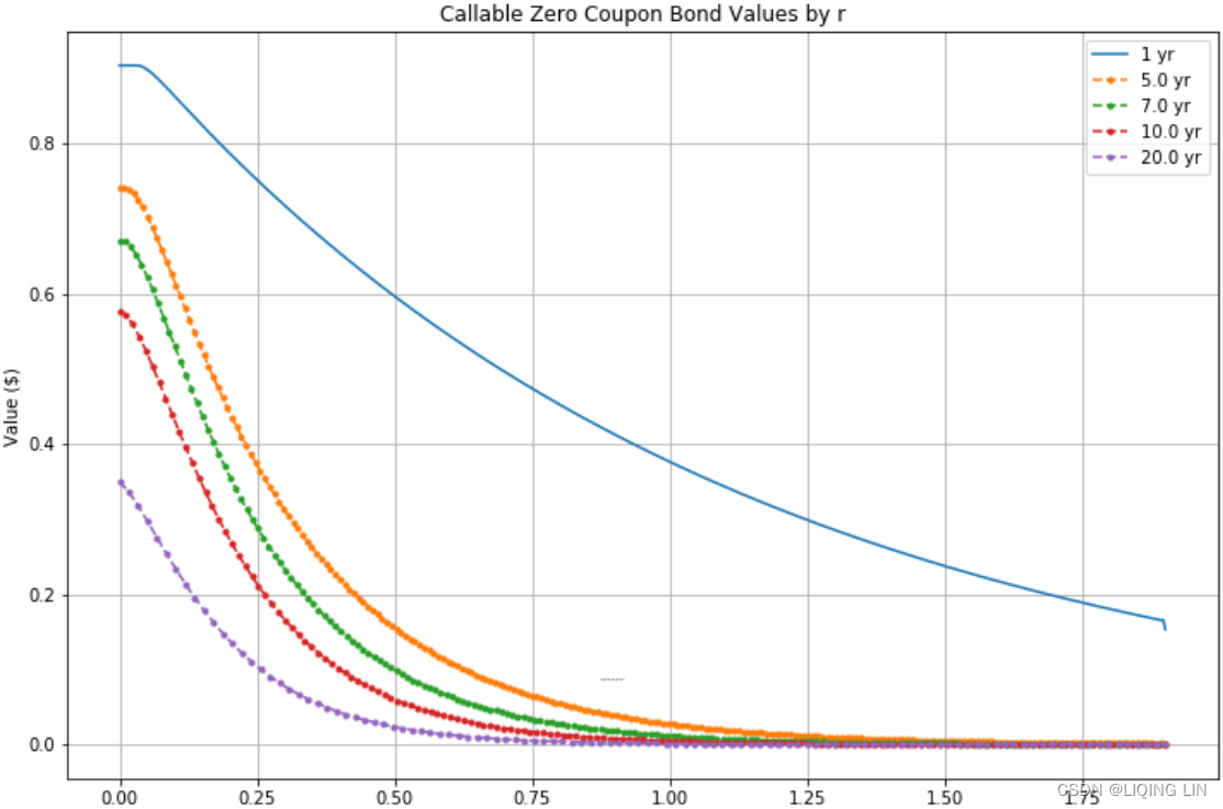

We obtained the theoretical values of pricing callable zero-coupon bonds for various maturities for various interest rates.

Other considerations in callable bond pricing

In pricing callable zero-coupon bonds, we used the Vasicek interest-rate process to model interest-rate movement with the aid of a normal distribution process. In The Vasicek model section, we demonstrated that the Vasicek model can produce negative interest rates, which may not be practical for most economic cycles. Quantitative analysts often use more than one model in derivative pricing to obtain realistic results. The CIR and Hull-White models are some of the commonly-discussed models in financial studies. The limitation on these models is that they involve only one factor, or a single source of uncertainty.

We also looked at the implicit scheme of finite differences for the policy iteration of the early exercise. Another method of consideration is the Crank-Nicolson method of finite differences. Other methods include the Monte Carlo simulation for calibration of this model.

Finally, we obtained a final list of short-rates and callable bond prices. To infer a fair value for the callable bond for a particular short-rate, interpolation of the list of bond prices is required. Often, the linear interpolation method is used. Other interpolation methods of consideration are the cubic and spline interpolation methods.

Summary

In this chapter, we focused on interest-rate and related derivative pricing with Python. Most bonds, such as US Treasury bonds, pay a fixed amount of interest semi-annually, while other bonds may pay quarterly or annually. It is a characteristic of bonds that their prices are closely related to current interest-rate levels in an inverse manner. The normal or positive yield curve, where long-term interest rates are higher than short-term interest rates, is said to be upward sloping. In certain economic conditions, the yield curve can be inverted and is said to be downward sloping(During periods of high inflation, where the inflation rate exceeds the rate of coupon interests, negative interest rates may be observed. Investors are willing to pay in the short-term just to secure their long-term wealth.).

A zero-coupon bond is a bond that pays no coupons during its lifetime, except upon maturity when the principal or face value is repaid. We implemented a simple zero-coupon bond calculator in Python.

The yield curve can be derived from the short-term zero or spot rates of securities, such as zero-coupon bonds, T-bills, notes, and eurodollar deposits using a bootstrapping process. With Python, we used a lot of bond information to plot a yield curve, and derived forward rates, yield-to-maturity, and bond prices from the yield curve.

Two important metrics to bond traders are duration and convexity. Duration(

$\large PV(C_t)=\frac{C_t}{(1+YTM)^t}$ OR $\large PV(C_t)=\frac{C_t + FV}{(1+YTM)^t}$ ==> $\large \frac{PV(C_t)}{BP}$ ==>

==>) is the sensitivity measure of bond prices to yield changes(Change in interest rates).
Convexity(think of convexity as the second derivative of the relationship between the price and yield) is the sensitivity measure of the duration of a bond to yield changes. We implemented calculations using the modified duration(Effective Duration
VS

) model and convexity calculator in Python.

Short-rate models are frequently used in the evaluation of interest-rate derivatives. Interest-rate modeling is a fairly complex topic, since they are affected by a multitude of factors, such as economic states, political decisions, government intervention, and the laws of supply and demand. A number of interest-rate models have been proposed to account for the various characteristics of interest rates. Some of the interest-rate models we discussed include the Vasicek(), CIR, and Rendleman and Bartter models.

Bond issuers may embed options within a bond to allow them the right, but not the obligation, to buy or sell the issued bond at a predetermined price during a specified period of time. The price of a callable bond can be thought of as the price difference of a bond
without an option and the price of the embedded call option.

Price of bond( Callable bonds holders'cost ) = price of bond with no option - price of embedded option

Price of puttable bond = price of bond with no option + price of put option

Using Python, we took a look at pricing a callable zero-coupon bond by applying the Vasicek model to the implicit method of finite differences.==> $\LARGE r_t = r_s e^{-K(t-s)} + \theta (1- e^{-K( t-s) } ) + \sigma \int_{s}^{t} e^{- K(t-u)} dw_u$ ==>
$\large P(t,T) = P(t,r,T) = A(t,T) e^{-r(t) B(t,T)}$ (2.3)
$\LARGE B(t,T) = \frac{1-e^{-K(T-t)}}{K}$ OR
$\large A(t,T) = e^{ ( \theta - \frac{ \sigma^2}{2K^2} ) ( B(t,T)-(T-t) ) - \frac{\sigma ^2}{4K} B^2(t,T) }$ OR
From (2.3), we are easy to obtain the following partial differential equation (PDE):

$\large \frac{\partial P_t}{\partial t} + K(\theta -r)\frac{\partial P_t}{\partial r} + \frac{1}{2}\sigma^2\frac{\partial^2 P_t}{\partial r^2} - rP_t =0$
with terminal condition $\large P(T,r,T)=1$ .

$\large rP_t = \frac{\partial P_t}{\partial t} + K(\theta -r)\frac{\partial P_t}{\partial r} + \frac{1}{2}\sigma^2\frac{\partial^2 P_t}{\partial r^2}$ This method is, however, just one of the many methods that quantitative analysts use in bond-options modeling.

In the next chapter, we will discuss the statistical analysis of time-series data.

LIQING LIN

关注

2
点赞
踩
6

收藏

觉得还不错? 一键收藏
0
评论
mpf5_定价Bond_yield curve_Spot coupon_duration_有效利率_连续复利_远期_Vasicek短期_CIR模型Derivatives_Tridiagonal_ppf

price Bond_yield curve_Spot rate Zero ratezero-coupon bond_bond duration and convexity_effective interest rate_Continuously compounded rate/interest_forward rates_effective interest rate_Vasicek model_Cox-Ingersoll model_Rendleman and Bartter model_Brenna.
复制链接

扫一扫